20171117 Notes: Stochastic Process, Parameter Estimation, PDE

This is the notes of Continuous Stochastic Structure Models with Apllication by Prof. Vijay S. Mookerjee. In this note, we are talking about Stochastic Process, Parameter Estimation, PDE and Stochastic Control.

Stochastic process

• Brownian Motion (BM): $Z_t \sim \mathcal{N}(0,t)$;
• Arithmetic Brownian Motion (ABM): $d \mu = \alpha dt + \sigma dZ_t$
• Geometric Brownian Motion (GBM): $dY_t = (\alpha + \frac{1}{2} \sigma^2) dt + \sigma dZ_t$
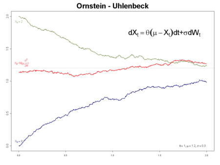
• Ornstein-Uhlenbeck process (O-U Process): $du = \alpha(\mu-u)dt + \sigma dZ_t$, where $\alpha$ is speed of reversion and $\mu$ is long-term mean (A.K.A steady state mean). The distribution of O-U Process is $u \sim \mathcal{N} (\mu_{\mathcal{N}}, \sigma_{\mathcal{N}})$, where $$\mu_{\mathcal{N}} = \mu + exp(-\alpha (X_0 - \mu))$$ $$\sigma_{\mathcal{N}} = \sigma^2 (1- \frac{exp(-2 \alpha t)}{2 \alpha}$$ As $t \rightarrow \infty$:
  • if $\alpha > 0$, $$lim_{t \to \infty} u \sim \mathcal{N} (\mu, \frac{\sigma^2}{2 \alpha})$$ Converge.
  • if $\alpha = 0$, $$lim_{t \to \infty} u \sim \mathcal{N} (\mu, \sigma^2 t)$$ Diverge.
  • if $\alpha < 0$, Diverge.

• Cox-Ingersoll-Ross (CIR) process: $dX_t = \alpha (\mu-X_t)dt+\sigma \sqrt{X_t} dZ_t$
• Stochastic Differential Equation for general 1-Spatial dimension Itô drift-diffusion process: $dX_t = \mu(X_t,t)dt + \sigma(X_t,t)dZ_t$
• Ito’s lemma: $Y$ is Itô drift-diffusion process, $f: \mathbb{R}^2 \to \mathbb{R}$ is smooth, then $$df(Y_t,t)=f_t dt + f_Y dY_t +\frac{1}{2} f_{YY} (dY_t)^2$$ $(dt)^2 = dt dW_t$; $(dW_t)^2 = dt$

Parameter Estimation

• Using Maximum Likelihood Estimation (MLE): $$\mathcal{L}(\theta|x) = f(x_1|\theta) \times f(x_2|\theta) \times \cdots \times f(x_n|\theta)$$ $$= f(x_1,x_2,\cdots,x_n|\theta) = \prod_{i=1}^{n} f(x_i|\theta)$$ $$\Rightarrow {\hat{\theta}_{MLE}} \subseteq { argmax_{\theta \in \Theta} \{ \hat{l}(\theta;x_1,x_2,\cdots,x_n) \} }$$
  • Exact MLE: Using known density function $f(x_i|\theta)$;
  • Inexact MLE:
    • First Difference Maximum Likelihood Estimation (FDMLE)¹
    • Fokker Planck Equation
• Fokker Planck Equation: $\frac{\partial}{\partial t} f(X_t,t) = - \frac{\partial}{\partial x}[\mu(X_t,t) \cdot f(X_t,t)]+\frac{1}{2}\frac{\partial^2}{\partial x^2}[\sigma^2(X_t,t) \cdot f(X_t,t)]$

Partial Differential Equation

• General linear second order Partial Differential Equation (PDE)²³: $$A u_{XX} +2B u_{XY} +C u_{YY} + D u_X +E u_Y + Fu =0$$
  • Elliptic: if $B^2-AC < 0$. Simple example is 2-D Laplace Equation: $u_{xx} + u_{yy}= 0$ (where $X = x$, $Y = y$, $A = 1$, $B = 0$, $C = 1$), which can describe the electrostatic field.
  • Parabolic: if $B^2-AC = 0$. Simple example is 1-D Heat Equation: $u_t - K u_{xx} = 0$ (where $X = x$, $Y = t$, $A = -K$, $B=C=0$), which can describe heat transportation process
    • Fokker Planck Equation: $$\frac{\partial}{\partial t} f(X_t,t) = - \frac{\partial}{\partial x}[\mu(X_t,t) \cdot f(X_t,t)]+\frac{1}{2}\frac{\partial^2}{\partial x^2}[\sigma^2(X_t,t) \cdot f(X_t,t)]$$
    • Black Scholes Eqaution: $$\frac{\partial V}{\partial t} + \frac{1}{2} \sigma^2 S^2 \frac{\partial^2 V}{\partial S^2} + rS \frac{\partial V}{\partial S} -rV = 0$$
  • Hyperbolic: if $B^2-AC > 0$. Simple example is 1-D Wave Equation: $a^2 u_{xx} - u_{tt} = 0$ (where $X = x$, $Y = t$, $A = a^2$, $B = 0$, $C = -1$), which can describe light wave.
• MATLAB function pdepe can solve initial-boundary value problems for parabolic-elliptic PDEs in 1-D.

Stochastic Optimal Control Process

• Stochastic Control problem concept:

  • Agent
  • State: $X_t$, SDE: $$d X_t = f(u, X, t) dt + g(u, X, t) dZ \tag{0}\label{0}$$
  • Control: $u(X_t,t)$
  • Objective Function: $F(u, t)$

• Using Brand Management on Twitter as an example:

  • Agent: Some firm, such as AT&T Co.
  • State: Sentiment Score of customers on Twitter;
  • Control: Effort AT&T Co. pay to increase the sentiment;
  • Objective Function: Return;

• If we want to minimize value function:

  $$V(X, t) = Min_{u(X, t)} \{F(u, t) dt + (1 - \gamma dt) V(X+dX, t+dt)\} \tag{1}\label{1}$$

  where $\gamma$ is discount factor.

• Taylor expansion on $\eqref{1}$:

  $$V(X+dX, t+dt) = V(t, X) + \frac{\partial V}{\partial X} dX + \frac{\partial V}{\partial t} dt + \frac{1}{2} (2 \frac{\partial^2}{\partial t \partial X} dtdX + \frac{\partial^2}{\partial t^2} (dt)^2 + \frac{\partial^2}{\partial X^2} (dX)^2) V$$ $$\stackrel{(dX)^2=g^2 dt}{=} V(t, X) + \frac{\partial V}{\partial X} dX + (\frac{\partial V}{\partial t} + \frac{g^2}{2} \frac{\partial^2 V}{\partial X^2}) dt$$ $$\stackrel{dX = fdt + gdZ}{=} V(t, X) + V_X (fdt + gdZ) + (V_t + \frac{g^2}{2} V_{XX}) dt$$ $$= V(t, X) + (fV_X + V_t + \frac{g^2}{2} V_{XX}) dt + g V_X dZ \tag{2}\label{2}$$
• $\eqref{2}$ into $\eqref{1}$: $$\gamma V dt = Min_{u(X, t)} \{F(u, t) dt + (f V_X + V_t + \frac{g^2}{2} V_{XX}) dt + g v_X dZ \} \tag{3}\label{3}$$
• Hamilton-Jacobi-Bellman (HJB) equation is a partial differential equation which is central to optimal control theory. The solution of the HJB equation is the value function which gives the minimum cost for a given dynamical system with an associated cost function.
  Expectation on $\eqref{3}$: $$\mathbb{E}[\gamma V dt] = Min_{u(X, t)} \mathbb{E} \{F(u, t) dt + (f V_X + V_t + \frac{g^2}{2} V_{XX}) dt + g v_X dZ\}$$ $$\stackrel{elim. dZ-term}{\Rightarrow} \gamma V dt = Min_{u(X, t)} \{F(u, t) dt + (f V_X + V_t + \frac{g^2}{2} V_{XX}) dt\}$$ $$\stackrel{HJB}{\Rightarrow} \gamma V= Min_{u(X, t)} \mathbb{E} \{F(u, t) + f V_X + V_t + \frac{g^2}{2} V_{XX}\} \tag{4}\label{4}$$
• Guess Objective Function (such as the return of the firm) follow the form of $F(u, t) = \beta X - C u^2$. Drift term of State $dX_t$ follow the form: $f(u, t) = k_1 u \sqrt{b-X} - k_2 X$; Volatility term of State $dX_t$ follow the form: $g(u, t) = k_3$. Thus replace $f$ and $g$ in $\eqref{4}$ HJB equation: $$\gamma V = Max_{u(X, t)} \{(\beta X - C u^2) + (k_1 u \sqrt{b-X} - k_2 X) V_X + V_t + \frac{k_3^2}{2} V_{XX}\} \tag{4*}\label{4*}$$
• Optimal Control: Partial derivative of the term inside $Max_{u(X, t)}$ in RHS w.r.t. $u$: $$\frac{(\beta X - C u^2) + (k_1 u \sqrt{b-X} - k_2 X) V_X + V_t + \frac{k_3^2}{2} V_{XX}}{\partial u} = 0$$ $$\Rightarrow -2Cu + V_X k_1 \sqrt{b-X} = 0$$ $$\Rightarrow u^* = \frac{V_X k_1 \sqrt{b-X}}{2C} \tag{5}\label{5}$$
• Guess $$V(x) = \lambda_1 X + \lambda_2 \tag{6}\label{6}$$ where $\lambda_1 > 0$, $V_X = \lambda_1$, $V_{XX} = V_t = 0$. Substitute $\eqref{5}$ and $\eqref{6}$ into $\eqref{4*}$: $$\gamma (\lambda_1 X + \lambda_2) = \beta X - \frac{\lambda_1^2 k_1^2 (b-X) C}{(2C)^2} + (k_1 \frac{\lambda_1 k_1 \sqrt{b-X}}{2C} \sqrt{b-X} - k_2 X) \lambda_1$$ $$= \beta X - \frac{\lambda_1^2 k_1^2 (b-X)}{4C} + (\frac{\lambda_1 k_1^2 (b-X)}{2C} - k_2 X) \lambda_1 \tag{7}\label{7}$$
• (X) part of $\eqref{7}$: $\gamma \lambda_1 = \beta - \frac{\lambda_1^2 k_1^2}{4C} - \lambda_1 k_2 \tag{8-1}\label{8-1}$
• (Constant) part of $\eqref{7}$: $\gamma \lambda_2 = \frac{\lambda_1^2 k_1^2}{4C} \tag{8-2}\label{8-2}$
• Solve $\eqref{8-1}$ and $\eqref{8-2}$ ($\lambda_1 > 0$): $$\lambda_1 = \frac{-2C(\gamma+k_2) + 2 \sqrt{C^2 (\gamma+k_2)^2 + C \beta k_1^2}}{k_1^2} \tag{9-1}\label{9-1}$$ $$\lambda_2 = \frac{\lambda_1^2 k_1^2 b}{4 \gamma C} \tag{9-2}\label{9-2}$$
• Substitute $\eqref{9-1}$ and $\eqref{9-2}$ in $\eqref{5}$: $$u^* = \frac{-C(\gamma+k_2) + \sqrt{C^2 (\gamma+k_2)^2 + C \beta k_1^2}}{k_1} \sqrt(b-X) \tag{10}\label{10}$$
• Substitute $\eqref{10}$ in $\eqref{0}$, note that $f(u, t) = k_1 u \sqrt{b-X} - k_2 X$, $g(u, t) = k_3$: $$dX = (-C(\gamma+k_2) + \sqrt{C^2 (\gamma+k_2)^2 + C \beta k_1^2} + k_2)$$ $$(\frac{b (-C(\gamma+k_2) + \sqrt{C^2 (\gamma+k_2)^2 + C \beta k_1^2})}{-C(\gamma+k_2) + \sqrt{C^2 (\gamma+k_2)^2 + C \beta k_1^2} + k_2} - X) dt + k_3 dZ \tag{11}\label{11}$$ Define: $$\alpha_{HJB} = -C(\gamma+k_2) + \sqrt{C^2 (\gamma+k_2)^2 + C \beta k_1^2} + k_2 \tag{12-1}\label{12-1}$$ $$\mu_{HJB} = \frac{b (-C(\gamma+k_2) + \sqrt{C^2 (\gamma+k_2)^2 + C \beta k_1^2})}{-C(\gamma+k_2) + \sqrt{C^2 (\gamma+k_2)^2 + C \beta k_1^2} + k_2} \tag{12-2}\label{12-2}$$ $$\sigma_{HJB} = k_3 \tag{12-3}\label{12-3}$$ Then $dX = \alpha_{HJB} (\mu_{HJB} - X) dt + \sigma_{HJB} dZ$, which is O-U process!
• According to O-U Process, state $X \sim \mathcal{N} (\mu_{\mathcal{N}}, \sigma_{\mathcal{N}})$, where $$\mu_{\mathcal{N}} = \mu_{HJB} + exp(-\alpha_{HJB} (X_0 - \mu_{HJB})) \tag{13-1}\label{13-1}$$ $$\sigma_{\mathcal{N}} = \sigma_{HJB}^2 (1- \frac{exp(-2 \alpha_{HJB} t)}{2 \alpha_{HJB}}) \tag{13-2}\label{13-2}$$ $X_t$ converge with $t \to \infty$ when $\eqref{12-1}$ $\alpha_{HJB} > 0$.

Read More

• MIT6.832 Lecture 16: Introducing Stochastic Optimal Control

• UTDallas-OPRE7320: Optimal Control Theory: Chap 13 Stochastic Optimal Control:

• Princeton-Economics 521, Advanced Macroeconomics I:

Lecture 4: Hamilton-Jacobi-Bellman Equations, Stochastic Differential Equations

Lecture 5: Stochastic HJB Equations, Kolmogorov Forward Equations

---

¹. Han, C., & Phillips, P. C. (2013). First difference maximum likelihood and dynamic panel estimation. Journal of Econometrics, 175(1), 35-45. ↩

². Partial Differential Equations in Finance ↩

³. Stanford MATH220a: 4 Classification of Second-Order Equations ↩