Textual Data
Headlines data
We use News Aggregator Data Set from UCI Machine Learning Repository. Headlines and categories for 400k news items scraped from the web in 2014. Columns are:
- ID : the numeric ID of the article
- TITLE : the headline of the article
- URL : the URL of the article
- PUBLISHER : the publisher of the article
- CATEGORY : the category of the news item; one of: — b : business — t : science and technology — e : entertainment — m : health
- STORY : alphanumeric ID of the news story that the article discusses
- HOSTNAME : hostname where the article was posted
- TIMESTAMP : approximate timestamp of the article’s publication, given in Unix time (seconds since midnight on Jan 1, 1970)
1 | # remove all the variables in the environment |
## [1] 422419 8
1 | names(data) |
## [1] "ID"        "TITLE"     "URL"       "PUBLISHER" "CATEGORY"  "STORY"
## [7] "HOSTNAME"  "TIMESTAMP"
1 | attach(data) |
## [1] 1 2 3 4 5
1 | head(TITLE,5) |
## [1] "Fed official says weak data caused by weather, should not slow taper"
## [2] "Fed's Charles Plosser sees high bar for change in pace of tapering"
## [3] "US open: Stocks fall after Fed official hints at accelerated tapering"
## [4] "Fed risks falling 'behind the curve', Charles Plosser says"
## [5] "Fed's Plosser: Nasty Weather Has Curbed Job Growth"
1 | head(URL,5) |
## [1] "http://www.latimes.com/business/money/la-fi-mo-federal-reserve-plosser-stimulus-economy-20140310,0,1312750.story\\?track=rss"
## [2] "http://www.livemint.com/Politics/H2EvwJSK2VE6OF7iK1g3PP/Feds-Charles-Plosser-sees-high-bar-for-change-in-pace-of-xfzta.html"
## [3] "http://www.ifamagazine.com/news/us-open-stocks-fall-after-fed-official-hints-at-accelerated-tapering-294436"
## [4] "http://www.ifamagazine.com/news/fed-risks-falling-behind-the-curve-charles-plosser-says-294430"
## [5] "http://www.moneynews.com/Economy/federal-reserve-charles-plosser-weather-job-growth/2014/03/10/id/557011"
1 | head(PUBLISHER,5) |
## [1] "Los Angeles Times" "Livemint"          "IFA Magazine"
## [4] "IFA Magazine"      "Moneynews"
1 | head(CATEGORY,5) |
## [1] "b" "b" "b" "b" "b"
1 | head(STORY,5) |
## [1] "ddUyU0VZz0BRneMioxUPQVP6sIxvM" "ddUyU0VZz0BRneMioxUPQVP6sIxvM"
## [3] "ddUyU0VZz0BRneMioxUPQVP6sIxvM" "ddUyU0VZz0BRneMioxUPQVP6sIxvM"
## [5] "ddUyU0VZz0BRneMioxUPQVP6sIxvM"
1 | head(HOSTNAME,5) |
## [1] "www.latimes.com"     "www.livemint.com"    "www.ifamagazine.com"
## [4] "www.ifamagazine.com" "www.moneynews.com"
1 | head(TIMESTAMP,5) |
## [1] 1.39447e+12 1.39447e+12 1.39447e+12 1.39447e+12 1.39447e+12
There are 422419 obervations in this dataset.
Time
The time of news range from 2014-03-10 16:52:50 GMT to 2014-08-28 12:33:11 GMT.
1 | mytime <- as.POSIXct(TIMESTAMP/1000, origin="1970-01-01", tz = "GMT") |
## [1] "2014-03-10 16:52:50 GMT" "2014-08-28 12:33:11 GMT"
Website
1 | #====== |
## [1] "www.latimes.com"     "www.livemint.com"    "www.ifamagazine.com"
## [4] "www.ifamagazine.com" "www.moneynews.com"   "www.nasdaq.com"
1 | data$WebSite<-wbsite |
##  [1] in.reuters.com              www.huffingtonpost.com
##  [3] www.businessweek.com        www.contactmusic.com
##  [5] www.dailymail.co.uk         www.nasdaq.com
##  [7] www.examiner.com            www.globalpost.com
##  [9] www.latimes.com             www.bizjournals.com
## [11] www.rttnews.com             thecelebritycafe.com
## [13] www.washingtonpost.com      www.entertainmentwise.com
## [15] www.forbes.com              www.bloomberg.com
## [17] www.nydailynews.com         www.marketwatch.com
## [19] time.com                    perezhilton.com
## [21] www.hngn.com                timesofindia.indiatimes.com
## [23] www.reuters.com             www.theguardian.com
## [25] www.telegraph.co.uk         www.wetpaint.com
## [27] au.ibtimes.com              blogs.wsj.com
## [29] www.techtimes.com           www.business-standard.com
## 11237 Levels: in.reuters.com www.huffingtonpost.com ... zumic.com
1 | # Output as csv |
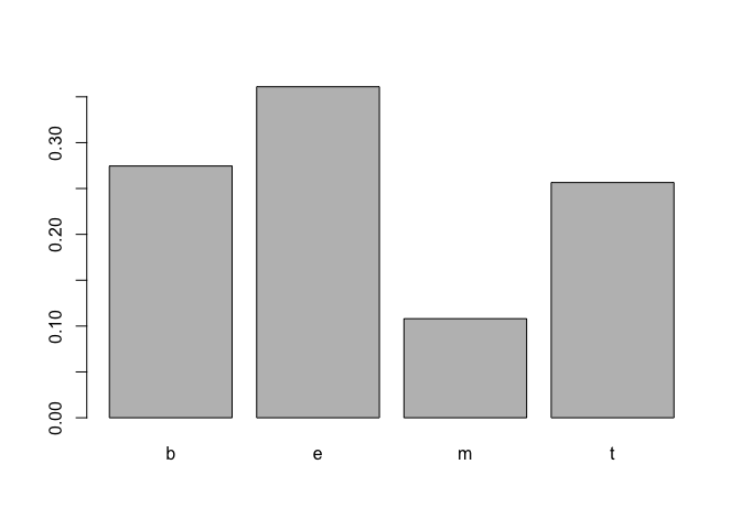
Category
There are:
- 152746 news of business category
- 108465 news of science and technology category
- 115920 news of business category
- 45615 news of health category
1 | table(CATEGORY) |
## CATEGORY
##      b      e      m      t
## 115967 152469  45639 108344
1 | # Freq plot |
Story
There are:
- 2076 clusters of similar news for entertainment category
- 1789 clusters of similar news for science and technology category
- 2019 clusters of similar news for business category
- 1347 clusters of similar news for health category
1 | # Business |
## [1] 2019 2
1 | # entertainment |
## [1] 2075 2
1 | # health |
## [1] 1347 2
1 | # science and technology |
## [1] 1789 2
Numerical Data
We use Dow Jones Industrial Average (DJIA) Index data here. And we collect the DJIA data from 2008-08-08 to 2016-07-01.
1 | DJIA<-read.csv("DJIA_table.csv",fill=T, sep=",", stringsAsFactors = FALSE) |
## [1] 1989 7
1 | names(DJIA) |
## [1] "Date"      "Open"      "High"      "Low"       "Close"     "Volume"
## [7] "Adj.Close"
1 | attach(DJIA) |
Date
1 | class(Date) |
## [1] "character"
1 | range(Date) |
## [1] "2008-08-08" "2016-07-01"
Close Price
1 | # Close Price |
##    Min. 1st Qu.  Median    Mean 3rd Qu.    Max.
##    6547   10913   13026   13463   16478   18312
1 | # Log Close Price |
##    Min. 1st Qu.  Median    Mean 3rd Qu.    Max.
##   8.787   9.298   9.475   9.479   9.710   9.815
1 | # Log Return |
##       Min.    1st Qu.     Median       Mean    3rd Qu.       Max.
## -0.1050835 -0.0057316 -0.0005430 -0.0002138  0.0045634  0.0820051
1 | # Histogram |
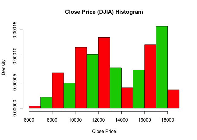
1 | hist(log_Close, freq=F, main="Log of Close Price (DJIA) Histogram", col=c(2,3), xlab="log(Close Price)") |

1 | hist(log_Return, freq=F, main="Log of Return (DJIA) Histogram", col=c(2,3), xlab="log(Return)") |
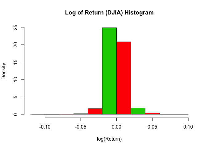
1 | # |
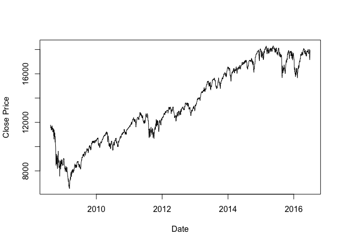
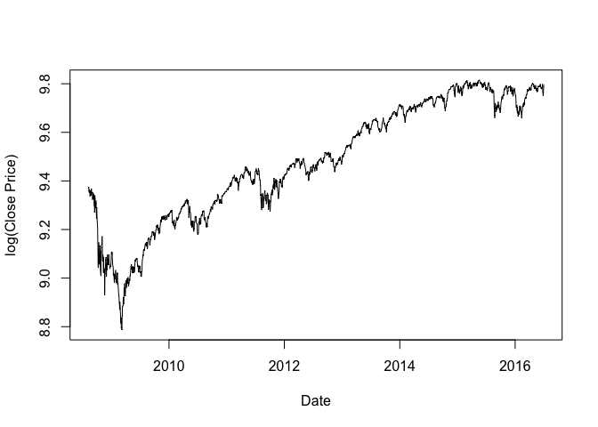
1 | plot(as.Date(Date), log_Close, type = "l", xlab = "Date", ylab = "log(Close Price)") |
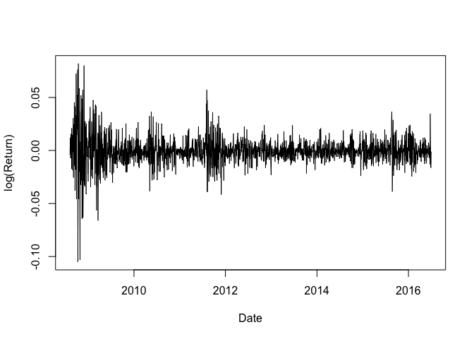
1 | plot(as.Date(Date[-1]), log_Return, type = "l", xlab = "Date", ylab = "log(Return)") |
