Preface
Nonlinear System is a system in which the change of the output is not proportional to the change of the input, which can modeled with a set of nonlinear equations. Solving the nonlinear equations can give us the clues of the behavior of a nonlinear system. Most of the time, the system is so complex that we can not solve it analytically but only numerically.
Assume there is a simple system of nonlinear equation:
And we need to solve it numerically. $\alpha$, $\beta$, $\lambda$, $\gamma$ are parameters.
The system of nonlinear equations can be written into myfun.m as follow:
1 | function F = myfun(var,para) |
To input parameters $\alpha$, $\beta$, $\lambda$, $\gamma$ into myfun, we can use para vector or global command in MATLAB. $\alpha$, $\beta$, $\lambda$, $\gamma$ are numerical data. When there are string type of data in parameters, we can use cell instead of vector.
If $\alpha \neq 0$ and $\lambda \neq 0$, then we can get four solutions as follow: $(x,y)=(-1,5)$, $(x,y)=(-1,-7)$, $(x,y)=(3,5)$, $(x,y)=(3,-7)$. Which one to be chosen depends on the initial condition. Thus initial condition is really important for solving system of nonlinear equations.
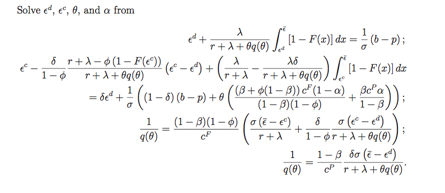
In most cases, the system of nonlinear equations that we would like to solve is really complicated that we can not even guess how the analytical solution could be. For example, if we want to solve $\epsilon^d$, $\epsilon^c$, $\theta$ and $alpha$ from the system of nonlinear equations as follow:
Parameters and functions $F(x)$ and $q (\theta)$ are stated as follow:

The functions $u$, $h_s$ and $h_n$ are defined as:

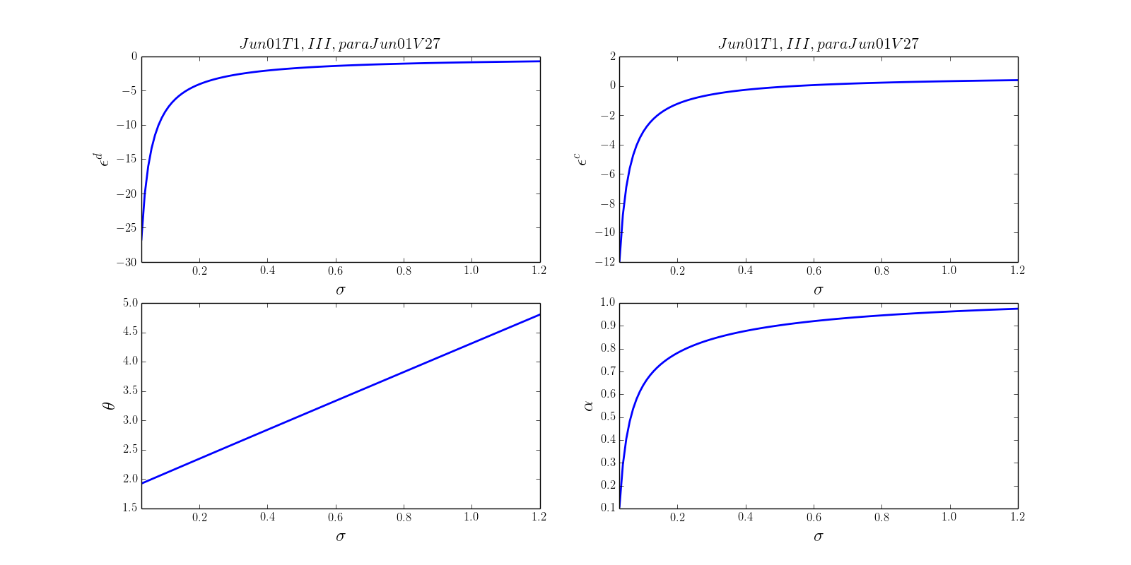
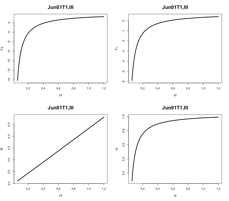
It should be emphasized that we also regard $\sigma$ as a variable. ($\sigma \in [0,0.5]$) Our final goal, we want to figure out the dynamic relationship of $\epsilon^d$, $\epsilon^c$, $\theta$, $alpha$ $\sim$ $\sigma$.
We are going to show how to solve this problem via using MATLAB, Fortran, Python and R.
MATLAB: fsolve, fmincon and lsqnonlin
In MATLAB, there are 3 kinds of solver to solve nonlinear equations: fsolve, fmincon and lsqnonlin.0
var vector represent $[\epsilon^d;\epsilon^c;\theta;\alpha]$.parameters vector represents $[c^F;c^p;\beta;\phi;\delta;\sigma;\lambda;b;r;\epsilon^c;\mu;step;width;typen]$.
We can define the nonlinear equation set as as follow:
1 | function F = fun_solveJun01T1(var,parameters) |
And we can also define function $F(x)$, $q(\theta)$, $u$, $h_s$ and $h_n$ as follow:
1 | F_x(i)=.5-.5*erf((log(-x(i)+1)+.5*log(2))/sqrt(2*log(2))); |
1 | function q_theta = fun_q_theta(theta,A,B1,B2) |
1 | function u = fun_u(epsilon_d,theta,lambda,typen,... |
1 | function h_s = fun_hs(epsilon_c,epsilon_d,theta,alpha,u,lambda,typen,... |
1 | function h_n = fun_hn(epsilon_c,theta,alpha,u,lambda,typen,... |
fsolve
Solves a problem specified by F(x) = 0 for x, where F(x) is a function that returns a vector value. x is a vector or a matrix; see Matrix Arguments.
fsolve is the most commonly used solver for nonlinear equations in MATLAB. In MATLAB, we can find three kinds of algorithms: Trust Region Dogleg1, Trust region and Levenberg-Marquardt.
We can set the options of solver fsolve as follow:
1 | options = optimoptions('fsolve'); |
The nonlinear equations that we want to solve are coded in function handle F.
1 | F = @(var)fun_solveJun01T1(var,para); |
And then we can solve nonlinear equation:
1 | [fs,~,exitflag] = fsolve(F,var0,options); |
where fs is the vector of solution and ceq is the value of nonlinear functions.
fmincon
Find minimum of constrained nonlinear multivariable function
For fmincon, there are 3 kinds of algorithms: Interior Point2, Trust Region Reflective3, Sequential Quadratic Programming (SQP)45, Active Set.
We can set the options as follow:
1 | options = optimoptions(@fmincon); |
We also need to set some constraint vectors following the suggested format of fmincon.
1 | Afmin=[];bfmin=[];Aeqfmin=[];beqfmin=[]; |
And then we can solve nonlinear equation:
1 | [fs,~,exitflag] = fmincon(@(var)0,var0,Afmin,bfmin,Aeqfmin,beqfmin,lbfmin,ubfmin,... |
where fun_solveJun01T1_nonlcon.m is as follow:
1 | function [c,ceq] = fun_solveJun01T1_nonlcon(var,para) |
lsqnonlin
Solve nonlinear least-squares (nonlinear data-fitting) problems
In lsqnonlin solver, Trust Region Reflective3 and Levenberg-Marquardt are used.
We can set the options as follow:
options = optimoptions(@lsqnonlin);
options.Algorithm = 'trust-region-reflective';
str_algo = 'TRR';
% 'trust-region-reflective' (default)
% A gradient to be supplied in the objective function
% 'levenberg-marquardt'
options.MaxFunctionEvaluations = Inf;
options.MaxIterations = 500;
We can also use function handle F to represent the nonlinear equations:
F = @(var)fun_solveJun01T1(var,para);
% var = [epsilon_d;epsilon_c;theta]
lblsq = [-Inf;-Inf;-Inf;-Inf];
if strcmp(typen,'I')
ublsq = [epsilon_u;epsilon_u;Inf;Inf];
else
ublsq = [epsilon_u;epsilon_u;Inf;Inf];
end
where lblsq and ublsp are the lower and upper bound.
Results
We can solve the equation Jun01T1 and get the solution for $\epsilon^d$, $\epsilon^c$, $\theta$ and $alpha$. In main.m:
1 | para ={A;B1;B2;c_f;c_p;beta;phi;delta;sigma;lambda;... |
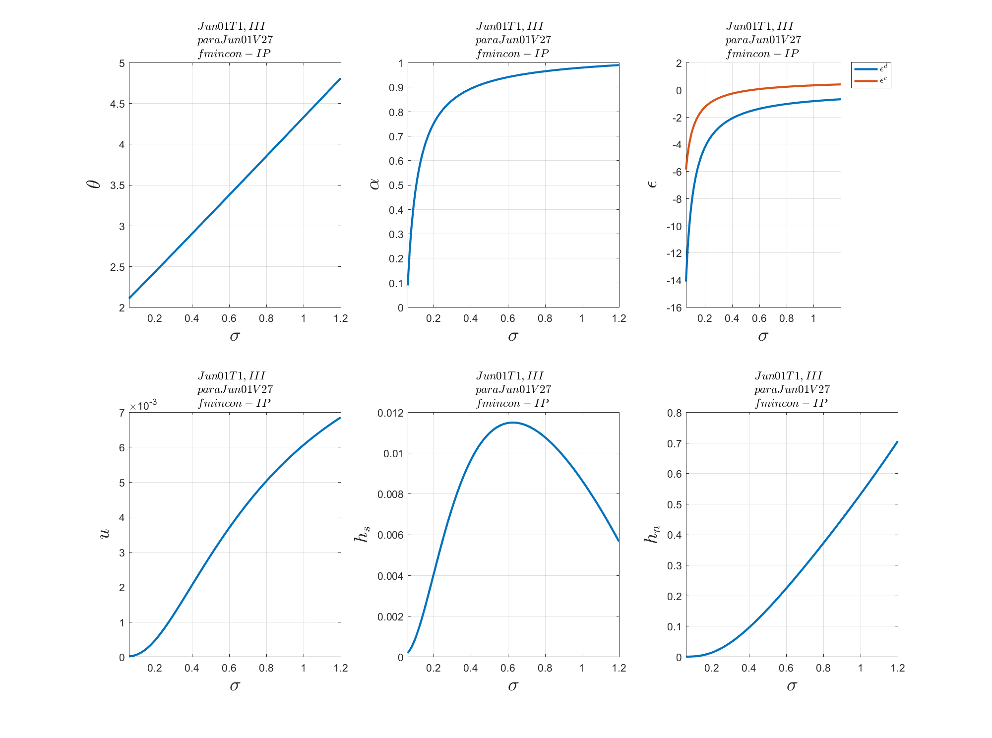
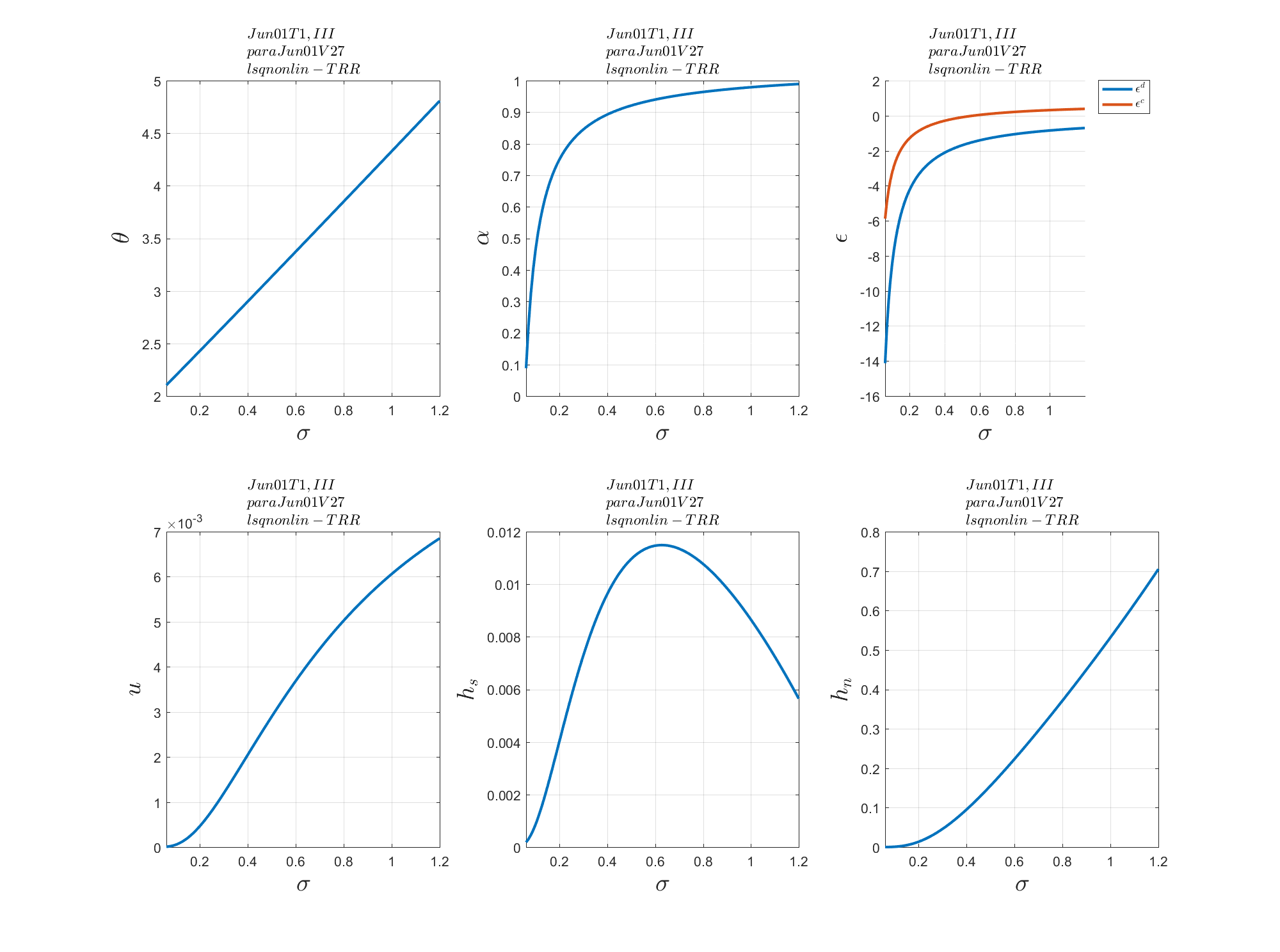
Then we can get plot the solution as follow
i. For the fsolve solver:

ii. For the fmincon solver:
iii. For the lsqnonlin solver:
Fortran: NEQNF
In IMSL Numerical Library, NEQNF can be used to solve a system of nonlinear equations by Powell’s Method, which uses finite-difference approximation to approximate Jacobian Matrix.
NEQNF
We can define the functions $u$, $h_s$ and $h_n$ in subroutines fun_u, fun_hs and fun_hn as follow:
1 | subroutine fun_u(epsilon_d,theta,u) |
1 | subroutine fun_hs(epsilon_c,epsilon_d,theta,alpha,u,h_s) |
1 | subroutine fun_hn(epsilon_c,theta,alpha,u,h_n) |
In subroutine Jun01T1, we can use CALL DNEQNF(FCN,ERRREL,N,ITMAX,XGUESS,X,fnorm) to solve system of nonlinear equations FCN.
1 | subroutine Jun01T1(epsilond,epsilonc,theta,alpha,exitflag) |
where subroutine FCN is defined as:
1 | subroutine FCN (X,F,N) |
In main.f90, we call the subroutine Jun01T1, fun_u, fun_hs and fun_hn:
1 | call Jun01T1(vepsilon_d(i),vepsilon_c(i),vtheta(i),valpha(i),vexitflag(i)) |
Results
Then we can plot the solutions as follow:

Python: fsolve in scipy.optimize package
We can use fsolve in scipy.optimize, which is a wrapper around [MINPACK’s hybrd and hybrj algorithms.
The purpose of HYBRD is to find a zero of a system of N non-linear functions in N variables by a modification of the Powell hybrid method. The user must provide a subroutine which calculates the functions. The Jacobian is then calculated by a forward-difference approximation.
The purpose of HYBRJ is to find a zero of a system of N non-linear functions in N variables by a modification of the Powell hybrid method. The user must provide a subroutine which calculates the functions and the Jacobian.
HYBRD is a modification of the Powell hybrid method. Two of its main characteristics involve the choice of the correction as a convex combination of the Newton and scaled gradient directions, and the updating of the Jacobian by the rank-1 method of Broyden.
fsolve in scipy.optimize
We define a Class named Operator to solve the nonlinear equations:
1 | class Operator(CaseCode): |
In the function Solution(self), we use fsolve in the format as follow:
1 | sol, infodict, ier, mesg = fsolve(self.Equation,guess,full_output=True) |
Results
We can take use of matplotlib.pyplot to plot the solutions as follow:
R: nleqslv package
To solve system of nonlinear equations, we can use nleqslv package. The nleqslv package provides two algorithms for solving (dense) nonlinear systems of equations:
- a Broyden Secant method6 where the matrix of derivatives is updated after each major iteration using the Broyden rank 1 update.
- a full Newton method where the Jacobian matrix of derivatives is recalculated at each iteration
nleqslv package
We can define the nonlinear Equations to be solved as follow:
1 | Equation<-function(x){ |
To solve the nonlinear equations, we can use nleqslv as follow:
1 | sol<-nleqslv(xstart,Equation,method="Broyden",control = list(trace=1)) |
Results
Taking use of the plot function in R, we can plot the solutions as follow:
Mathematica: Export results as image or .m file
Generally, we can use NSolve in Mathematica to solve system of nonlinear equations. However, it really takes time to handle with the nonlinear equations that we want to solve. But there are a few useful techniques that I would like to cover here.
Export result as images
We can define the function $F(x)$ and $q(\theta)$ as follow:
1 | funqtheta[\[Theta]_, A_, B_] := A*\[Theta]^(-B); |
We can also define the system of nonlinear equations and variables as follow:
1 | part11 = \[Epsilon]d + \[Lambda]* |
Then we can calculate the Jacobian Matrix as follow:
1 | (* Jacobian Matrix *) |
We can export the results of partial derivatives as images:
1 | Simplify[ArrayReshape[Jac[[All, 1]], {4, 1}]] // TraditionalForm |
Export as MATLAB file
Or we can take use of the Wolfram Library ToMatlab to convert the results into MATLAB .m files as follow:
1 | WriteMatlab[Jac[[All, 1]], "dF_depsilond.m", "dF_depsilond", 50] |
For example, dF_depsilond.m file is as follow
1 | function dF_depsilond=dF_depsilond_fun(A,B1,B2,mu,epsilon_u,... |
ToMatlab in Mathematica can really make MATLAB much more powerful because of the better analytical capacity of Mathematica compared with MATLAB.
Results
The exported image of partial derivatives, such as $\frac{\partial F}{\partial \epsilon^d}$, is as follow:

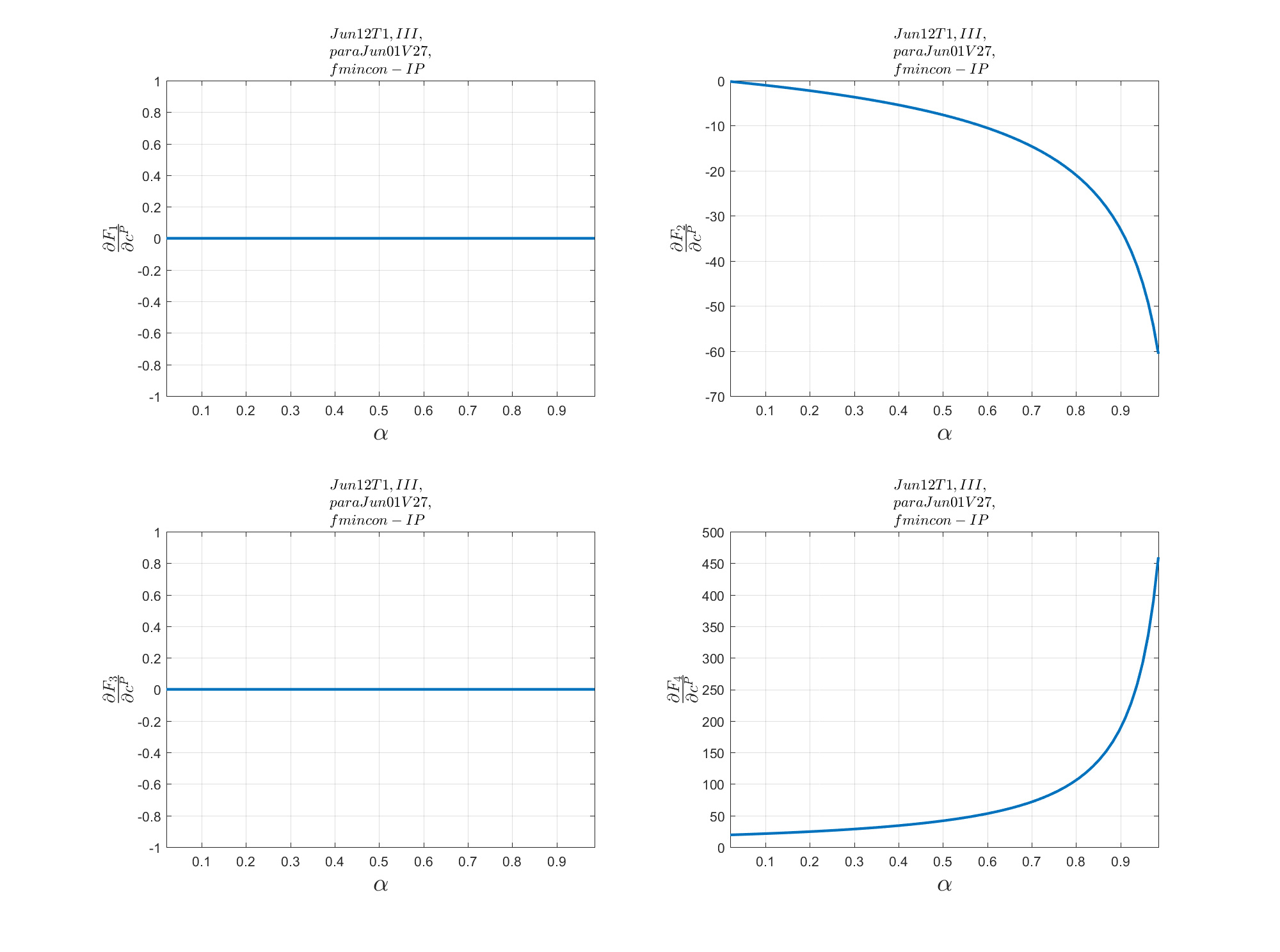
We can plot the dynamics between partial derivatives and some variables (such as $\alpha$) as follow:
More: To ODE and PDE
System of Nonlinear Equation has big relationship with Ordinary Differential Equations (ODE) and Partial Differential Equations (PDE) in numerical analysis. And there are so many famous nonlinear equations out there in various disciplines.7 Thus knowing how to solve nonlinear equations numerically is crucial in mathematical modeling in different aspects.
0. MathWork:Nonlinear Systems with Constraints ↩
1. Lecture 7: The Dogleg and Steihaug Methods ↩
2. Interior-point method for NLP ↩
3. Trust Region Reflective Algorithm ↩
4. Constrained Nonlinear Optimization Algorithms ↩
5. Nocedal, J., & Wright, S. (2006). Numerical optimization. Springer Science & Business Media. ↩
6. Broyden’s method ↩
7. Some famous nonlinear equations ↩
