Model

In this post, we use Monte Carlo simulations to validate the Fama-French five-factor model and the O.L.S properties. We confirm the validity of five factors in the Fama-French model, and uncover some interesting findings of O.L.S properties.

Wikipedia: Fama–French model

$r - R_f = \beta_1 + \beta_2 (K_m - R_f) + \beta_3 \cdot SMB + \beta_4 \cdot HML + \beta_5 \cdot RMW + \beta_6 \cdot CMA$

$r$ is the portfolio’s expected rate of return
$R_f$ is the risk-free return rate
$K_m$ is the return of the market portfolio

The “five factor” $\beta_2$ to $\beta_6$ are:

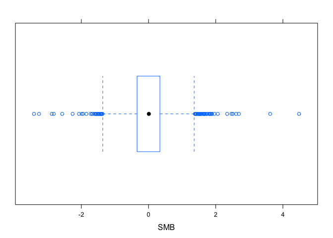
SMB (Small [market capitalization] Minus Big) is the average return on the nine small stock portfolios minus the average return on the nine big stock portfolios;
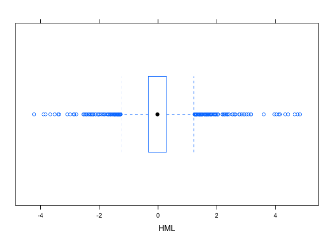
HML (High [book-to-market ratio] Minus Low) is the average return on the two value portfolios minus the average return on the two growth portfolios;
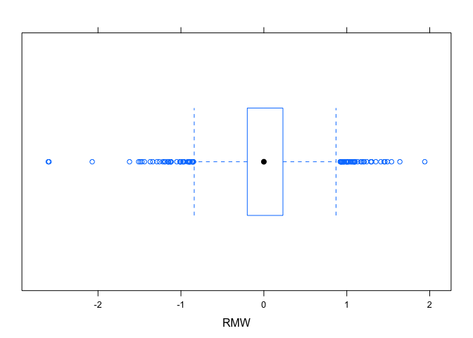
RMW (Robust Minus Weak) is the average return on the two robust operating profitability portfolios minus the average return on the two weak operating profitability portfolios;
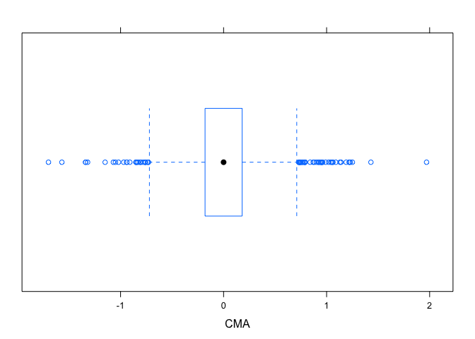
CMA (Conservative Minus Aggressive) is the average return on the two conservative investment portfolios minus the average return on the two aggressive investment portfolios.

They measure the historic excess returns of small caps over big caps and of value stocks over growth stocks.

These factors are calculated with combinations of portfolios composed by ranked stocks (BtM ranking, Cap ranking) and available historical market data. Historical values may be accessed on Kenneth French’s web page.

Here is Description of Fama/French 5 Factors (2x3)

Data Source

Data is downloaded from homepage of Kenneth R. French.

Fama/French 3 Factors [Daily]

This file was created by CMPT_ME_BEME_RETS using the 201801 CRSP database. The 1-month TBill return is from Ibbotson and Associates, Inc.

Portfolios Formed on Book-to-Market [Daily]

This file was created by CMPT_BEME_RETS_DAILY using the 201801 CRSP database. It contains value- and equal-weighted returns for portfolios formed on BE/ME. The portfolios are constructed at the end of June. BE/ME is book equity at the last fiscal year end of the prior calendar year divided by ME at the end of December of the prior year. The annual returns are from January to December. Missing data are indicated by -99.99 or -999. The break points use Compustat firms plus the firms hand-collected from the Moodys Industrial, Utilities, Transportation, and Financial Manuals. The break points include utilities. The portfolios use Compustat firms plus the firms hand-collected from the Moodys Industrial, Utilities, Transportation, and Financial Manuals. The portfolios include utilities.

These portfolios are created by doing the following:

Rank all stocks that trade on NYSE, Nasdaq and Amex (when it existed) by their book-to-marketratios
Take the bottom 30% and put them into a portfolio (low 30%)
Take the next 40% and put them into a portfolio (medium 40%)
Take the top 30% and put them into a portfolio (top 30%)
Portfolio weights within each portfolio are value-weights

Load Data

Here is our data:

rm(list=ls())
# Load data file into R
load(file="5factors_2008_2018.RData")
dim(mydata2)

## [1] 2518   26

Extract Fama-French Factors and Fund Returns

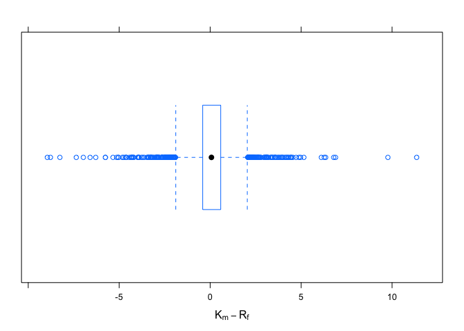
rmrf: K_m − R_f
smb: SMB
hml: HML
rmw: RMW
cma: CMA
rf: R_f
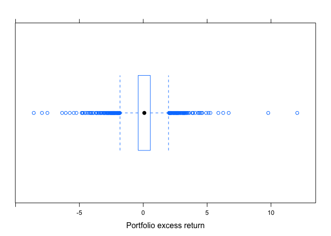
lo_30: r, the portfolio’s expected rate of return. Here, we choose the portfolio with firms of lowest 30% value- and equal-weighted returns.

Now, we extract Fama-French Factors and Fund Returns from dataset:

1 2	mydate <- mydata2$Date range(mydate)

## [1] "2008-01-02" "2017-12-29"

rmrf <- mydata2$Mkt.RF
smb <- mydata2$SMB
hml <- mydata2$HML
rf <- mydata2$RF
rmw <- mydata2$RMW
cma <- mydata2$CMA

The, we calculate Excess Returns for Target fund

1	lo_30.xcess <- mydata2$Lo.30 - rf

Run Fama-French Regression

Plot of data:

#=========================
### Boxplots
library(lattice)
bwplot(~lo_30.xcess, xlab = "Portfolio excess return") # Both side outliers

1	bwplot(~rmrf, xlab = expression(K[m] - R[f]))

1	bwplot(~smb, xlab = "SMB")

1	bwplot(~hml, xlab = "HML")

1	bwplot(~rmw, xlab = "RMW")

1	bwplot(~cma, xlab = "CMA")

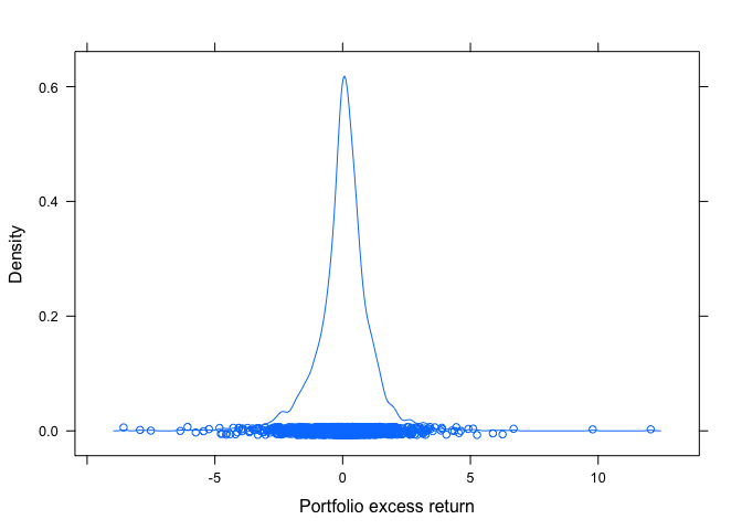
1 2	# density plot densityplot(lo_30.xcess, xlab = "Portfolio excess return")

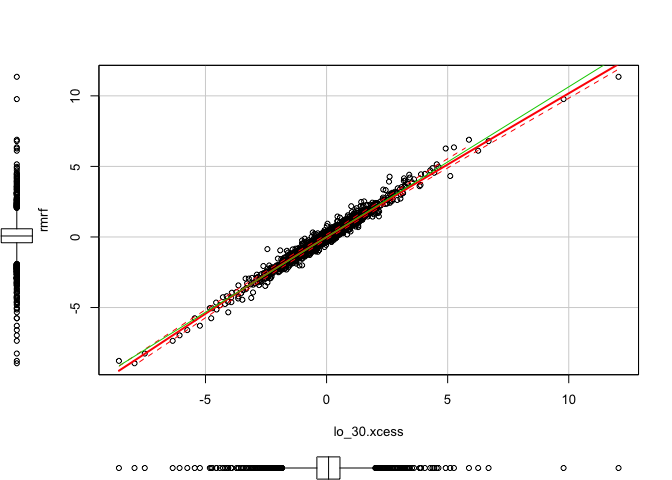
1 2	library(car) # red line affected by outlier, green ignoring the outlier (robust) scatterplot(x = lo_30.xcess, y = rmrf) #(dependent)

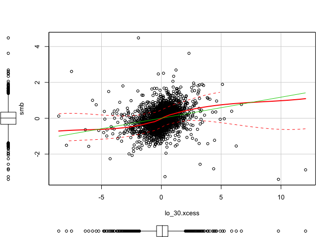
1	scatterplot(x = lo_30.xcess, y = smb) #(dependent)

1	scatterplot(x = lo_30.xcess, y = hml) #(dependent)

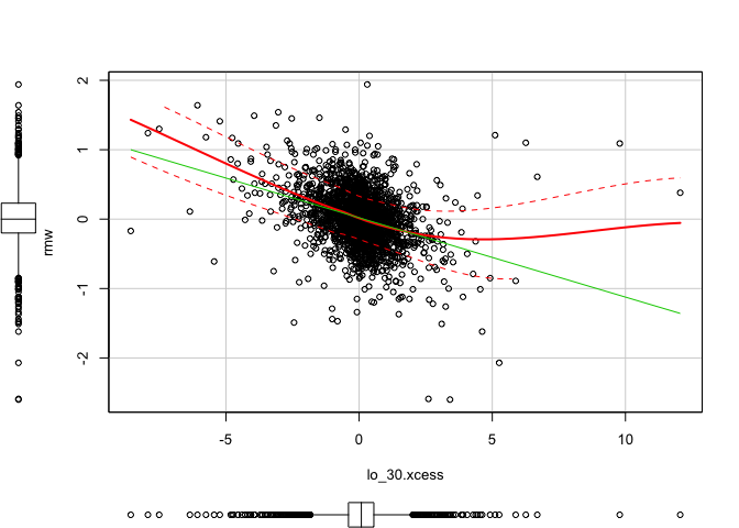
1	scatterplot(x = lo_30.xcess, y = rmw) #(dependent)

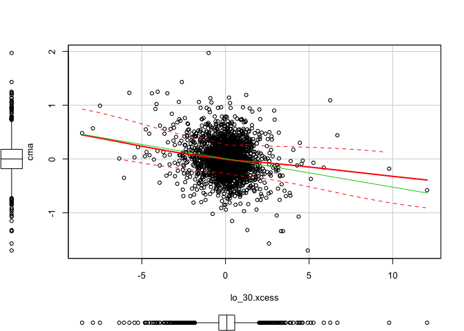
1	scatterplot(x = lo_30.xcess, y = cma) #(dependent)

library(ggplot2)
# scatterplot using ggplot
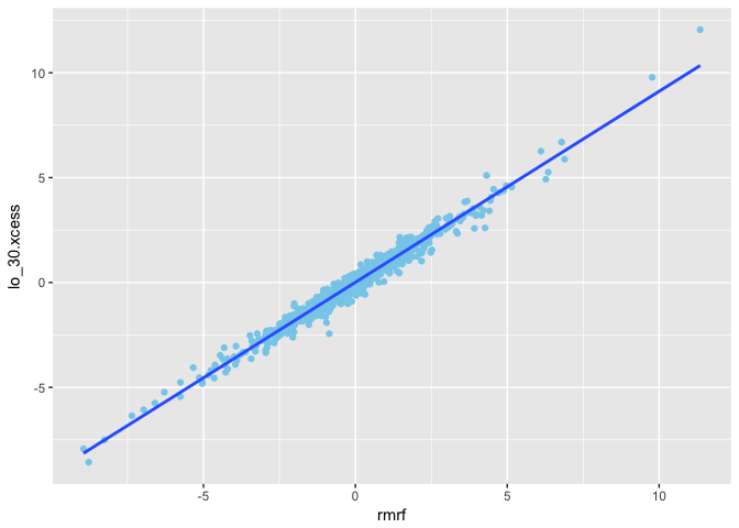
ggplot(mapping = aes(x = rmrf, y = lo_30.xcess)) + 
  geom_point(colour = 'skyblue') + 
  geom_smooth(method = 'lm')

1
2
3

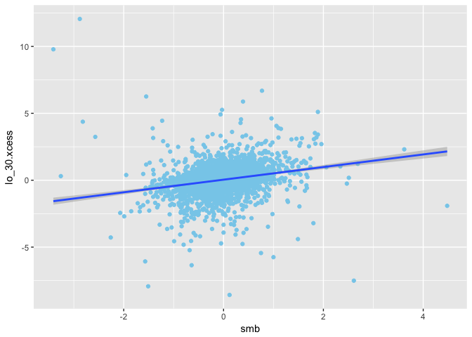
ggplot(mapping = aes(x = smb, y = lo_30.xcess)) + 
  geom_point(colour = 'skyblue') + 
  geom_smooth(method = 'lm')

1
2
3

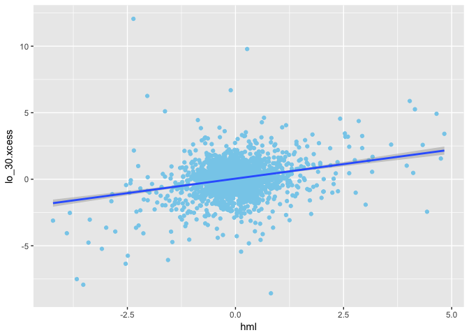
ggplot(mapping = aes(x = hml, y = lo_30.xcess)) + 
  geom_point(colour = 'skyblue') + 
  geom_smooth(method = 'lm')

1
2
3

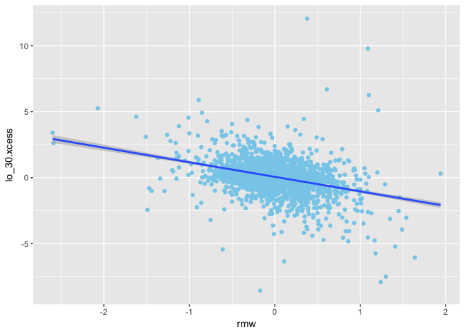
ggplot(mapping = aes(x = rmw, y = lo_30.xcess)) + 
  geom_point(colour = 'skyblue') + 
  geom_smooth(method = 'lm')

1
2
3

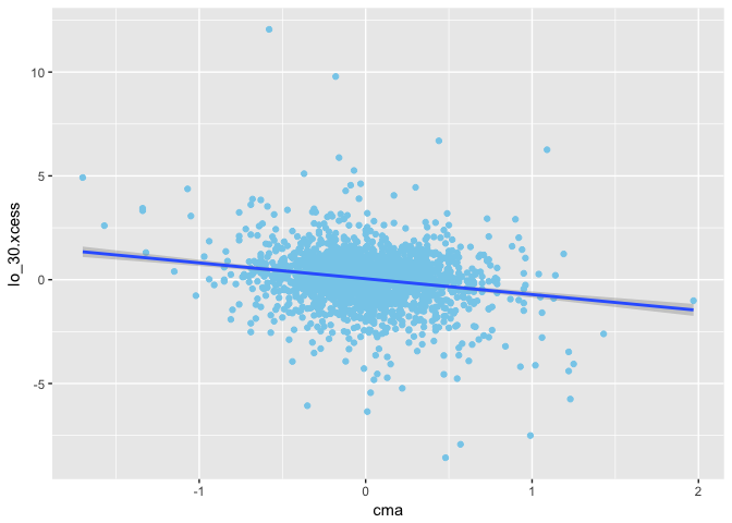
ggplot(mapping = aes(x = cma, y = lo_30.xcess)) + 
  geom_point(colour = 'skyblue') + 
  geom_smooth(method = 'lm')

We can run the linear regression to get the β.

lo_30.ffregression <- lm(lo_30.xcess ~ 
                           rmrf + smb + hml + rmw + cma)
# Print summary of regression results
lo_30.sum <- summary(lo_30.ffregression)
lo_30.sum

## 
## Call:
## lm(formula = lo_30.xcess ~ rmrf + smb + hml + rmw + cma)
## 
## Residuals:
##      Min       1Q   Median       3Q      Max 
## -0.59616 -0.05422 -0.00001  0.05556  0.52712 
## 
## Coefficients:
##              Estimate Std. Error t value Pr(>|t|)    
## (Intercept)  0.004495   0.001949   2.306   0.0212 *  
## rmrf         0.979197   0.001806 542.072  < 2e-16 ***
## smb         -0.029402   0.003511  -8.374  < 2e-16 ***
## hml         -0.258457   0.003373 -76.618  < 2e-16 ***
## rmw          0.055243   0.006215   8.889  < 2e-16 ***
## cma         -0.034451   0.006684  -5.154 2.74e-07 ***
## ---
## Signif. codes:  0 '***' 0.001 '**' 0.01 '*' 0.05 '.' 0.1 ' ' 1
## 
## Residual standard error: 0.09759 on 2512 degrees of freedom
## Multiple R-squared:  0.9933, Adjusted R-squared:  0.9933 
## F-statistic: 7.486e+04 on 5 and 2512 DF,  p-value: < 2.2e-16

Plot of regression:

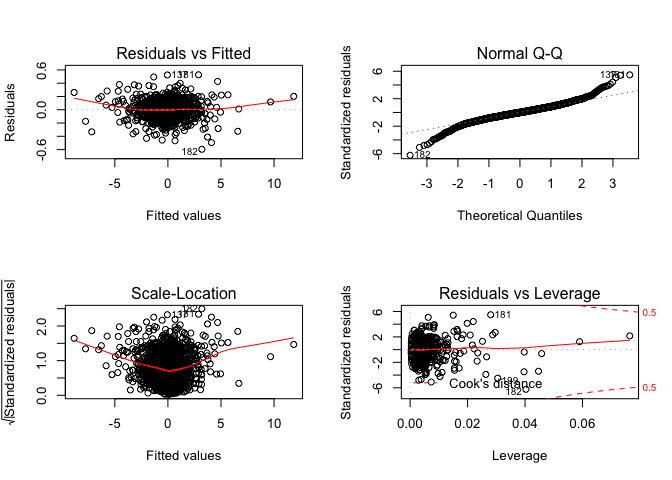
1 2	par(mfrow=c(2,2)) plot(lo_30.ffregression)

Monte Carlo Simulation

Next, we are running Monte Carlo Simulation for Fama French 5 Factor Model.

#===========================================
## Construct X data frame
# X data: rmrf, smb, hml, rmw, cma
X <- data.matrix(cbind(rep(1, dim(mydata2)[1]), 
                       rmrf, smb, hml, rmw, cma))
is.matrix(X)

## [1] TRUE

dim(X)

## [1] 2518    6

# # obervations
M <- dim(X)[1]
# True beta
beta <- lo_30.sum$coefficients[,1]
is.vector(beta)

## [1] TRUE

1	class(beta)

## [1] "numeric"

1	length(beta)

## [1] 6

#
mu <- 0
sig2e <- var(lo_30.xcess)
# True sigma: std of distribution of error term
sde <- sqrt(sig2e)
sde

## [1] 1.194133

One example of Monte Carlo Simulation

1
2
3

set.seed(12345)
Y <- X %*% beta + rnorm(M, mean=0, sd=sde)
class(Y)

## [1] "matrix"

1	is.vector(Y)

## [1] FALSE

1	is.matrix(Y)

## [1] TRUE

length(Y)

## [1] 2518

ff<-lm(Y~X[,-1])

sum <- summary(ff)
sum

## 
## Call:
## lm(formula = Y ~ X[, -1])
## 
## Residuals:
##     Min      1Q  Median      3Q     Max 
## -3.9939 -0.7897  0.0157  0.8026  3.9580 
## 
## Coefficients:
##              Estimate Std. Error t value Pr(>|t|)    
## (Intercept) -0.002067   0.023685  -0.087    0.930    
## X[, -1]rmrf  0.980129   0.021947  44.659  < 2e-16 ***
## X[, -1]smb  -0.067441   0.042660  -1.581    0.114    
## X[, -1]hml  -0.308533   0.040985  -7.528 7.14e-14 ***
## X[, -1]rmw  -0.056562   0.075507  -0.749    0.454    
## X[, -1]cma  -0.023310   0.081204  -0.287    0.774    
## ---
## Signif. codes:  0 '***' 0.001 '**' 0.01 '*' 0.05 '.' 0.1 ' ' 1
## 
## Residual standard error: 1.186 on 2512 degrees of freedom
## Multiple R-squared:  0.503,  Adjusted R-squared:  0.502 
## F-statistic: 508.5 on 5 and 2512 DF,  p-value: < 2.2e-16

#==============================
# Confidence interval
cfi<-confint(ff)
cfi

##                   2.5 %      97.5 %
## (Intercept) -0.04851118  0.04437665
## X[, -1]rmrf  0.93709258  1.02316506
## X[, -1]smb  -0.15109374  0.01621131
## X[, -1]hml  -0.38890087 -0.22816575
## X[, -1]rmw  -0.20462411  0.09150049
## X[, -1]cma  -0.18254382  0.13592330

1	class(cfi)

## [1] "matrix"

dim(cfi)

## [1] 6 2

# If true beta is in confidence interval of estimated beta
flag.beta <- logical(length(beta))
for (k in 1:length(beta)){
flag.beta[k] <- cfi[k,1]<=beta[k]&&cfi[k,2]>=beta[k]
}
flag.beta

## [1] TRUE TRUE TRUE TRUE TRUE TRUE

1	class(flag.beta)

## [1] "logical"

1	length(flag.beta)

## [1] 6

#==============================
# estimated error variance
err.var <- deviance(ff)/df.residual(ff)
err.var

## [1] 1.405962

1
2
3

#==============================
# \hat{\beta}
ff$coefficients

##  (Intercept)  X[, -1]rmrf   X[, -1]smb   X[, -1]hml   X[, -1]rmw 
## -0.002067263  0.980128819 -0.067441217 -0.308533310 -0.056561812 
##   X[, -1]cma 
## -0.023310260

#==============================
# T-Test: Null Hypothesis: betahat = beta
# Significant level of t-test
alp <- 0.05
# T statistics = (betahat-beta)/s.e.
t.stat <- (sum$coefficients[,1]-beta)/sum$coefficients[,2]
# t_{1-\alpha/2, n-k}
thr <- qt(1-alp/2, df = df.residual(ff))
# whether reject null hypothesis: False - not reject; True - reject (Type I)
# We should not reject the null hypothesis of beta = betahat
# But if we reject it (<alp), we are making Type I error, right?
flag.type1 <- t.stat>thr | t.stat < - thr
flag.type1

## (Intercept) X[, -1]rmrf  X[, -1]smb  X[, -1]hml  X[, -1]rmw  X[, -1]cma 
##       FALSE       FALSE       FALSE       FALSE       FALSE       FALSE

1	class(flag.type1)

## [1] "logical"

1	length(flag.type1)

## [1] 6

Running Monte Carlo Simulation

Run the Monte Carlo Simulation as follow.

Note:

this is just a demo with replication number N = 100.
Actually, we run the Monte Carlo Simulation with replication number N = 10⁵
We will save the data in a file named mcff5_2008_2018.RData.

# level of t-test
alpha <- 0.05
#
temp <- 1:length(beta)
nbv <- temp[-2]
# Number of Replication
N <- 100
mat.beta <- matrix(0,nrow = N, ncol = length(beta))
mat.beta2 <- matrix(0,nrow = N, ncol = length(beta)-1)
vec.flag.beta <- logical(N*length(beta))
vec.err.var <- numeric(N)
vec.err.var2 <- numeric(N)
vec.flag.type1 <- logical(N*length(beta))
vec.flag.type1.2 <- logical(N*(length(beta)-1))
mat.t.stat <- matrix(0,nrow = N, ncol = length(beta))
mat.t.stat2 <- matrix(0,nrow = N, ncol = length(beta)-1)
# 
for (i in 1:N) {
  set.seed(27+6*i)
  Y <- X %*% beta + rnorm(M, mean=0, sd=sde)
  # Full Linear Regression
  ff<-lm(Y~X[,-1])
  # Omitt rmrf variable
  ff2<-lm(Y~X[,c(-1,-2)])
  # Confidence interval
  cfi<-confint(ff)
  # If true: beta is in confidence interval of estimated beta
  for (k in 1:length(beta)){
    vec.flag.beta[(i-1)*length(beta)+k] <- 
      cfi[k,1]<=beta[k]&&cfi[k,2]>=beta[k]
  }
  # estimated error variance
  vec.err.var[i] <- deviance(ff)/df.residual(ff)
  vec.err.var2[i] <- deviance(ff2)/df.residual(ff2)
  # \hat{\beta}
  mat.beta[i,] <- as.matrix(ff$coefficients)
  mat.beta2[i,] <- as.matrix(ff2$coefficients)
  # T statistics = (betahat-beta)/s.e.
  sum <- summary(ff)
  sum2 <- summary(ff2)
  mat.t.stat[i,] <- (sum$coefficients[,1]-beta)/
    sum$coefficients[,2]
  mat.t.stat2[i,] <- (sum2$coefficients[,1]-beta[nbv])/
    sum2$coefficients[,2]
  # t_{1-\alpha/2, n-k}
  threshold <- qt(1-alpha/2, df = df.residual(ff))
  # whether reject null hypothesis: False - not reject; True - reject (Type I)
  # We should not reject the null hypothesis of beta = betahat
  # But if we reject it (<alp), we are making Type I error, right?
  for (k in 1:length(beta)){
    vec.flag.type1[(i-1)*length(beta)+k] <-
      mat.t.stat[i,k] > threshold | 
      mat.t.stat[i,k] < -threshold
  }
  for (k in 1:(length(beta)-1)){
    vec.flag.type1.2[(i-1)*(length(beta)-1)+k] <- 
      mat.t.stat2[i,k] > threshold | 
      mat.t.stat2[i,k] < -threshold
  }
}
mat.flag.beta <- matrix(vec.flag.beta, 
                        ncol = length(beta), 
                        byrow = T)
mat.flag.type1 <- matrix(vec.flag.type1, 
                         ncol = length(beta), 
                         byrow = T)
mat.flag.type1.2 <- matrix(vec.flag.type1.2, 
                           ncol = length(beta)-1, 
                           byrow = T)

Plot

Load the completed Monte Carlo data from file and set the parameters.

rm(list=ls())
#graphics.off()
#=======================================================================================#
# load data
load(file="5factors_2008_2018.RData")
# Extract Fama-French Factors and Fund Returns
mydate <- mydata2$Date
range(mydate)

## [1] "2008-01-02" "2017-12-29"

rmrf <- mydata2$Mkt.RF
smb <- mydata2$SMB
hml <- mydata2$HML
rf <- mydata2$RF
rmw <- mydata2$RMW
cma <- mydata2$CMA

# Calculate Excess Returns for Target fund
lo_30.xcess <- mydata2$Lo.30 - rf
#==================================================
# Run Fama-French Regression
lo_30.ffregression <- lm(lo_30.xcess ~ 
                           rmrf + smb + hml + rmw + cma)
# Print summary of regression results
lo_30.sum <- summary(lo_30.ffregression)
#===========================================
## Construct X data frame
# X data: rmrf, smb, hml, rmw, cma
X <- data.matrix(cbind(rep(1, dim(mydata2)[1]), 
                       rmrf, smb, hml, rmw, cma))
# Coloum Summary
summaryfun <- function(x){
  nr = dim(x)[2]
  nc = 6
  temp <- rep(NA, nr*nc)
  out <- matrix(temp, nrow = nr, ncol = nc) 
  for (i in 1:dim(X)[2]){
    out[i,] <- c(N = length(x[,i]),
                 Mean = mean(x[,i]),
                 Median = median(x[,i]),
                 StdDev = sd(x[,i]),
                 Min = min(x[,i]),
                 Max = max(x[,i]))
  }
  out1 <- as.data.frame(out)
  return(out1)
}
des.stat <- summaryfun(X)
names(des.stat) <- c("N",
                     "Mean", 
                     "Median",
                     "St.Dev",
                     "Min",
                     "Max")
row.names(des.stat) <- c("1",
                             "RmRf", 
                             "SMB",
                             "HML",
                             "RMW",
                             "CMA")
# stargazer
#install.packages("stargazer") #Use this to install it, do this only once
library(stargazer)

## 
## Please cite as:

##  Hlavac, Marek (2018). stargazer: Well-Formatted Regression and Summary Statistics Tables.

##  R package version 5.2.1. https://CRAN.R-project.org/package=stargazer

1	stargazer(as.data.frame(X), type = "text", title="Descriptive statistics", digits=4, out="output_star_X.txt")

## 
## Descriptive statistics
## ===============================================
## Statistic   N    Mean  St. Dev.   Min     Max  
## -----------------------------------------------
## V1        2,518 1.0000  0.0000     1       1   
## rmrf      2,518 0.0410  1.2911  -8.9500 11.3500
## smb       2,518 0.0080  0.5957  -3.4100 4.4800 
## hml       2,518 0.0002  0.7224  -4.2200 4.8300 
## rmw       2,518 0.0139  0.3843  -2.6000 1.9400 
## cma       2,518 0.0030  0.3146  -1.7000 1.9700 
## -----------------------------------------------

# # obervations
M <- dim(X)[1]
# True beta
beta <- lo_30.sum$coefficients[,1]
#
mu <- 0
sig2e <- var(lo_30.xcess)
# True sigma: std of distribution of error term
sde <- sqrt(sig2e)

#==================================
# Load runned data
load(file = "mcff5_2008_2018_mutiplemodel_20180403.RData")
attach(object)
dim(object)

## NULL

#===========================
# Significance level of t-test
alpha <- 0.05
# Ordinal number for second model with omitted variable
temp <- 1:length(beta)
nbv2 <- temp[-2]
nbv3 <- temp[-3]
nbv4 <- temp[-4]
nbv5 <- temp[-5]
nbv6 <- temp[-6]
nbv7 <- temp[1:4]
nbv8 <- temp[1:2]
#=======================
#vecN = c(10,50,100)
vecN = c(10,50,100,500,1e3,5e3,seq(from = 1e4, to = 1e5, by = 1e4))
mat.betahat <- matrix(0, 
                      nrow = length(vecN), 
                      ncol = length(beta))
mat.betahat2 <- matrix(0, 
                       nrow = length(vecN), 
                       ncol = length(nbv2))

mat.vebh <- matrix(0, 
                   nrow = length(vecN), 
                   ncol = length(beta))
vec.err.varh <- numeric(length(vecN))
vec.prob.err.varh <- numeric(length(vecN))
vec.err.varh2 <- numeric(length(vecN))
vec.prob.err.varh2 <- numeric(length(vecN))
prob.flag.beta <- matrix(0, 
                         nrow = length(vecN), 
                         ncol = length(beta))
prob.flag.type1 <- matrix(0, 
                          nrow = length(vecN), 
                          ncol = length(beta))
prob.flag.type1.2 <- matrix(0, 
                            nrow = length(vecN), 
                            ncol = length(beta)-1)
mat.t.stathat <- matrix(0, 
                        nrow = length(vecN), 
                        ncol = length(beta))
for (j in 1:length(vecN)){
  N <- vecN[j]
  # tolerance
  epsilon <- 0.05
  # \hat{\beta}
  mat.betahat[j,] <- colMeans(mat.beta[1:N,])
  #
  mat.betahat2[j,] <- colMeans(mat.beta2[1:N,])
  # \variance of betahat
  mat.vebh[j,] <- apply(mat.beta[1:N,], 2, var)
  # error variance
  vec.err.varh[j] <- mean(vec.err.var[1:N])
  # P(abs(err.varh - sig2e) >= epsilon)
  vec.prob.err.varh[j] <- sum(abs(vec.err.var[1:N] - sig2e) 
                              >= epsilon)/N
  # error variance for model 2
  vec.err.varh2[j] <- mean(vec.err.var2[1:N])
  # P(abs(err.varh - sig2e) >= epsilon)
  vec.prob.err.varh2[j] <- sum(abs(vec.err.var2[1:N] - sig2e) 
                               >= epsilon)/N
  # Probability of true beta is in confidence interval of estimated beta
  prob.flag.beta[j,] <- colSums(mat.flag.beta[1:N,])/N
  # Prob of Type I
  prob.flag.type1[j,] <- colSums(mat.flag.type1[1:N,])/N
  # Prob of Type I
  prob.flag.type1.2[j,] <- colSums(mat.flag.type1.2[1:N,])/N
  # 
  mat.t.stathat[j,] <- colMeans(mat.t.stat[1:N,])
}
#==============================================
# Model Selection Table
v.rsq.adj <- c(mean(rsq.adj),mean(rsq.adj2),mean(rsq.adj3),mean(rsq.adj4),
           mean(rsq.adj5),mean(rsq.adj6),mean(rsq.adj7),mean(rsq.adj8))
v.aic <- c(mean(aic),mean(aic2),mean(aic3),mean(aic4),
           mean(aic5),mean(aic6),mean(aic7),mean(aic8))
v.bic <- c(mean(bic),mean(bic2),mean(bic3),mean(bic4),
           mean(bic5),mean(bic6),mean(bic7),mean(bic8))
v.mlcp <- c(NaN,mean(mlcp2),mean(mlcp3),mean(mlcp4),
           mean(mlcp5),mean(mlcp6),mean(mlcp7),mean(mlcp8))
model_select <- as.data.frame(cbind(v.rsq.adj,
                              v.aic,
                              v.bic,
                              v.mlcp))
names(model_select) <- c("Adjusted R-squared", 
                       "AIC",
                       "BIC",
                       "Mallow's Cp")
row.names(model_select) <- c("Full Model",
                             "Model 2",
                             "Model 3",
                             "Model 4",
                             "Model 5",
                             "Model 6",
                             "Model 7",
                             "Model 8")
#sink("output_model_select.txt")
print(model_select)

##            Adjusted R-squared      AIC      BIC  Mallow's Cp
## Full Model          0.4982286 8046.163 8086.981          NaN
## Model 2             0.1064741 9498.768 9533.756 1963.3724737
## Model 3             0.4981351 8045.635 8080.622   -0.5302520
## Model 4             0.4903992 8084.166 8119.153   38.2578132
## Model 5             0.4981208 8045.706 8080.694   -0.4588785
## Model 6             0.1064741 8045.325 8080.312   -0.8401955
## Model 7             0.4980998 8044.814 8073.970    0.6473720
## Model 8             0.4863740 8100.990 8118.484   61.5142284

#sink()
#==============================================
# Table of Probability of Type I error for different model
temp <- rep(NA, 8*length(beta))
prob.type1 <- matrix(temp,nrow = 8, ncol = length(beta)) 
prob.type1[1,]<- colSums(mat.flag.type1)/tail(toN,1)
prob.type1[2,nbv2] <- colSums(mat.flag.type1.2)/tail(toN,1)
prob.type1[3,nbv3] <- colSums(mat.flag.type1.3)/tail(toN,1)
prob.type1[4,nbv4] <- colSums(mat.flag.type1.4)/tail(toN,1)
prob.type1[5,nbv5] <- colSums(mat.flag.type1.5)/tail(toN,1)
prob.type1[6,nbv6] <- colSums(mat.flag.type1.6)/tail(toN,1)
prob.type1[7,nbv7] <- colSums(mat.flag.type1.7)/tail(toN,1)
prob.type1[8,nbv8] <- colSums(mat.flag.type1.8)/tail(toN,1)
prob.type1 <- as.data.frame(prob.type1)
names(prob.type1) <- c("beta1", 
                         "beta2", 
                         "beta3", 
                         "beta4", 
                         "beta5", 
                         "beta6")
row.names(prob.type1) <- c("Full Model",
                             "Model 2",
                             "Model 3",
                             "Model 4",
                             "Model 5",
                             "Model 6",
                             "Model 7",
                             "Model 8")
#sink("output_prob_typeI.txt")
print(prob.type1)

##              beta1   beta2   beta3   beta4   beta5   beta6
## Full Model 0.04988 0.05079 0.04952 0.05018 0.05194 0.04833
## Model 2    0.29885      NA 0.99999 1.00000 1.00000 1.00000
## Model 3    0.04979 0.05161      NA 0.05018 0.05478 0.04849
## Model 4    0.04823 0.59559 0.08615      NA 0.69012 0.64035
## Model 5    0.04969 0.05283 0.05521 0.05892      NA 0.04890
## Model 6    0.04976 0.05202 0.04929 0.05418 0.05192      NA
## Model 7    0.04977 0.05082 0.05601 0.07178      NA      NA
## Model 8    0.04872 0.95811      NA      NA      NA      NA

#sink()
#==============================================
# Difference between simulated value and true value
temp <- rep(NA, 
            8*(length(beta) + 1))
tab.bias <- matrix(temp,nrow = 8, 
                   ncol = length(beta) + 1) 
tab.bias[1,] <- c(
  # Bias of OLS estmator of beta
  abs(beta-colMeans(mat.beta)),
  # Bias of OLS estimator of Error Variance
  abs(sig2e-mean(vec.err.var)))
tab.bias[2,c(nbv2,7)] <- c(
  # Bias of OLS estmator of beta
  abs(beta[nbv2]-colMeans(mat.beta2)),
  # Bias of OLS estimator of Error Variance
  abs(sig2e-mean(vec.err.var2)))
tab.bias[3,c(nbv3,7)] <- c(
  # Bias of OLS estmator of beta
  abs(beta[nbv3]-colMeans(mat.beta3)),
  # Bias of OLS estimator of Error Variance
  abs(sig2e-mean(vec.err.var3)))
tab.bias[4, c(nbv4,7)] <- c(
  # Bias of OLS estmator of beta
  abs(beta[nbv4]-colMeans(mat.beta4)),
  # Bias of OLS estimator of Error Variance                    
  abs(sig2e-mean(vec.err.var4)))
tab.bias[5, c(nbv5,7)] <- c(
  # Bias of OLS estmator of beta
  abs(beta[nbv5]-colMeans(mat.beta5)),
  # Bias of OLS estimator of Error Variance                    
  abs(sig2e-mean(vec.err.var5)))
tab.bias[6, c(nbv6,7)] <- c(
  # Bias of OLS estmator of beta
  abs(beta[nbv6]-colMeans(mat.beta6)),
  # Bias of OLS estimator of Error Variance                    
  abs(sig2e-mean(vec.err.var6)))
tab.bias[7, c(nbv7,7)] <- c(
  # Bias of OLS estmator of beta
  abs(beta[nbv7]-colMeans(mat.beta7)),
  # Bias of OLS estimator of Error Variance                    
  abs(sig2e-mean(vec.err.var7)))
tab.bias[8, c(nbv8,7)] <- c(
  # Bias of OLS estmator of beta
  abs(beta[nbv8]-colMeans(mat.beta8)),
  # Bias of OLS estimator of Error Variance                    
  abs(sig2e-mean(vec.err.var8)))
tab.bias <- as.data.frame(tab.bias)
names(tab.bias) <- c("beta1", 
                       "beta2", 
                       "beta3", 
                       "beta4", 
                       "beta5", 
                       "beta6",
                     "Error Variance")
row.names(tab.bias) <- c("Full Model",
                           "Model 2",
                           "Model 3",
                           "Model 4",
                           "Model 5",
                           "Model 6",
                           "Model 7",
                           "Model 8")
#sink("output_table_bias.txt")
print(tab.bias)

##                   beta1        beta2        beta3        beta4
## Full Model 5.097693e-05 4.548356e-06 0.0001277153 0.0000584728
## Model 2    4.978255e-02           NA 0.3205085589 0.6105273388
## Model 3    3.617108e-04 2.554723e-03           NA 0.0025626935
## Model 4    2.947476e-04 4.621952e-02 0.0247329253           NA
## Model 5    8.998804e-04 3.272899e-03 0.0083072828 0.0110698879
## Model 6    1.948356e-04 2.363134e-03 0.0014945671 0.0061072960
## Model 7    7.339447e-04 1.141030e-03 0.0090608459 0.0156089053
## Model 8    3.142667e-03 6.844190e-02           NA           NA
##                   beta5        beta6 Error Variance
## Full Model 0.0001093913 0.0001619033   4.572658e-05
## Model 2    0.6890978267 0.9219254461   1.113663e+00
## Model 3    0.0136155417 0.0041033581   2.201317e-04
## Model 4    0.1751336438 0.1788627543   2.221245e-02
## Model 5              NA 0.0060159119   2.605182e-04
## Model 6    0.0032572051           NA   4.449708e-05
## Model 7              NA           NA   3.202380e-04
## Model 8              NA           NA   3.365506e-02

#sink()

Plot of density of estimator

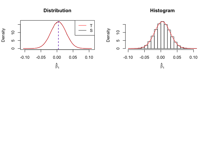
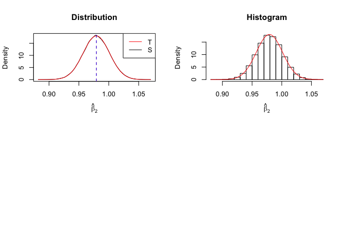
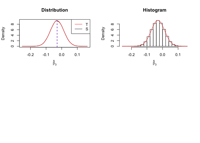
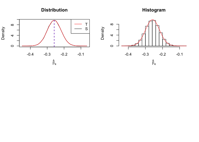
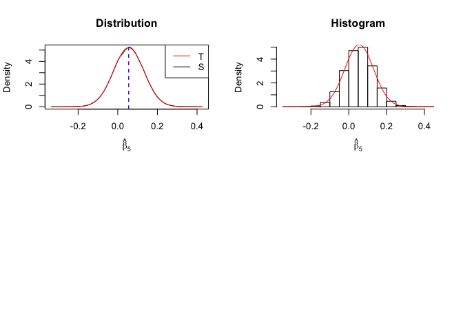
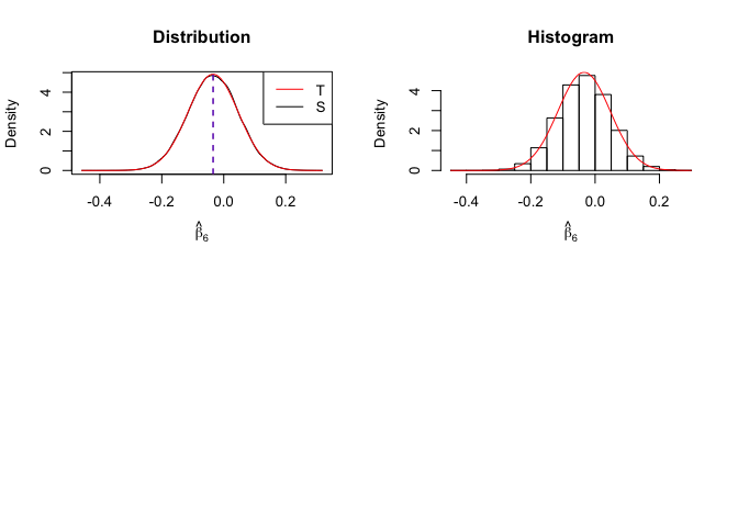
Number of replication N = 10⁵

# In Distribution pic, blue line is true beta, red line is betahat
foo = expression(hat(beta)[1], hat(beta)[2],hat(beta)[3],
                 hat(beta)[4],hat(beta)[5],hat(beta)[6])
for (i in 1:length(beta)){
  # mypath <- file.path(getwd(),"Figure",paste("density_beta_",i, ".jpeg", sep = ""))
  # jpeg(mypath, height = 8, width = 8, units = 'in', res = 300)
  # beta_{i}
  par(mfrow=c(2,2))
  plot(density(mat.beta[,i]), 
       xlab = foo[[i]], 
       main = "Distribution")
  curve(dnorm(x, mat.betahat[length(vecN),i], 
              sqrt(mat.vebh[length(vecN),i])), 
        col="red", add=TRUE)
  abline(v=mat.betahat[length(vecN),i], 
         col = "red", lty = 2)
  abline(v=beta[i], col = "blue", lty = 2)
  # "T" for "True", "S" for "Simulated"
  legend("topright", legend=c("T", "S"), 
         lty=1, col=c("red", "black"))
  # dev.off()
  ##
  # mypath <- file.path(getwd(),"Figure",paste("hist_beta_",i, ".jpeg", sep = ""))
  # jpeg(mypath, height = 8, width = 8, units = 'in', res = 300)
  hist(mat.beta[,i], prob=TRUE, 
       xlab = foo[[i]], 
       main = "Histogram")
  curve(dnorm(x, mat.betahat[length(vecN),i], 
              sd=sqrt(mat.vebh[length(vecN),i])), 
        col="red", 
        add=TRUE)
  # "T" for "True", "S" for "Simulated"
  # legend("topright", legend=c("T", "S"), 
  #        lty=1, col=c("red", "black"))
  # dev.off()
}

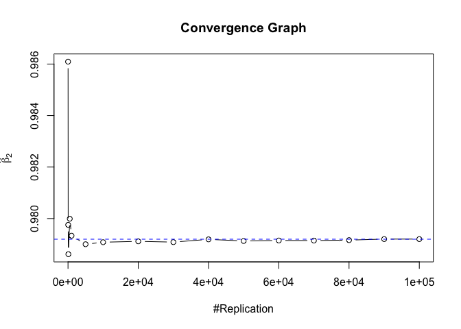
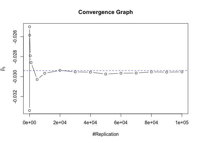
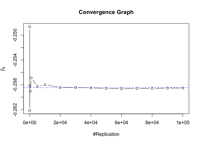
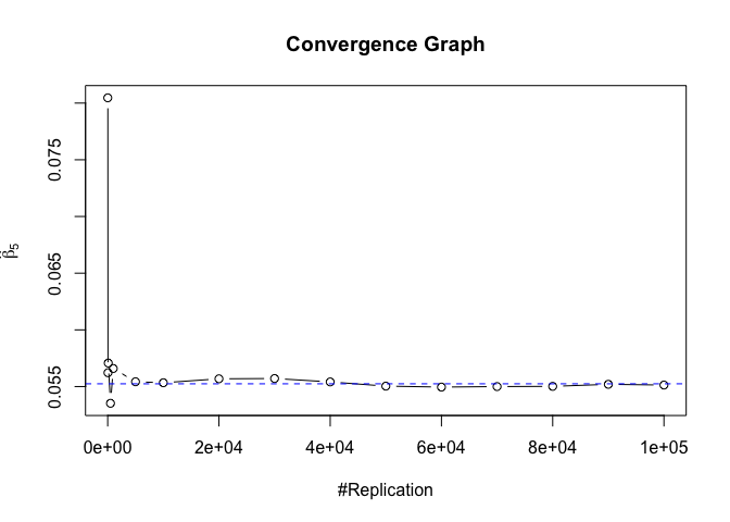
Finding (i)

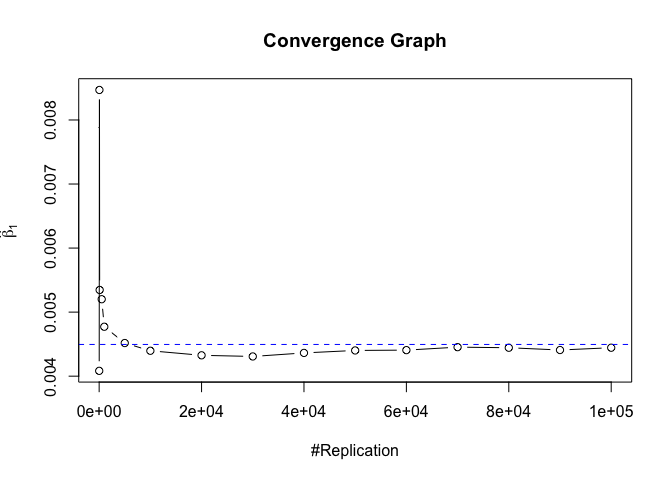
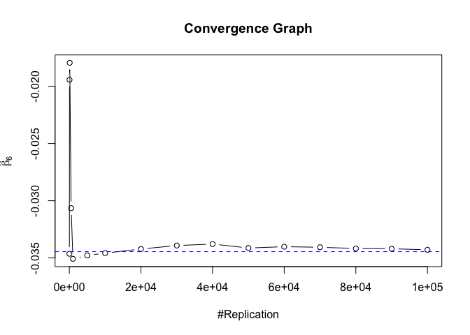
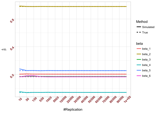
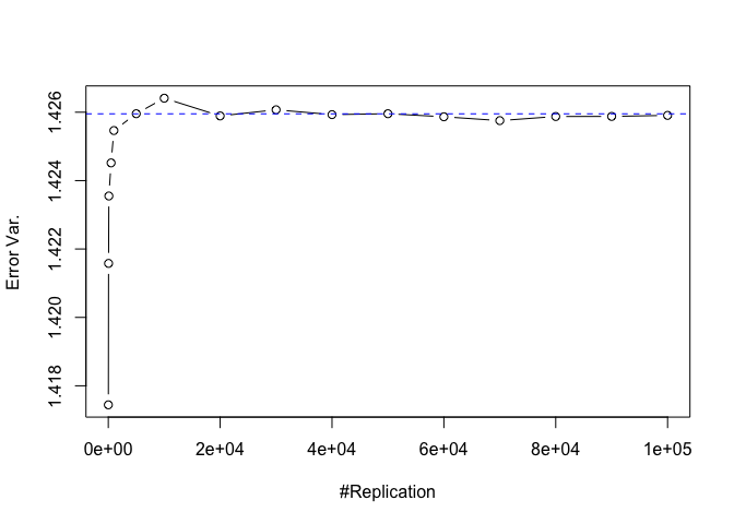
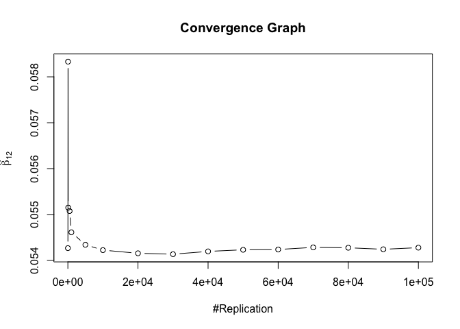
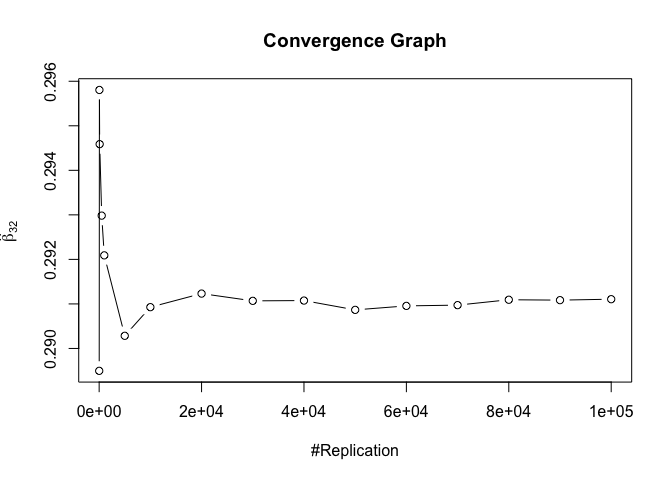
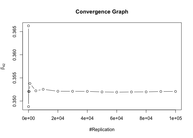
The O.L.S. estimators of the unknown coefficients and error variance are unbiased

Plot of betahat

foo = expression(hat(beta)[1], hat(beta)[2],hat(beta)[3],
                 hat(beta)[4],hat(beta)[5],hat(beta)[6])
for (i in 1:length(beta)){
  # mypath <- file.path(getwd(),"Figure",paste("i_OLS_betahat_",i, ".jpeg", sep = ""))
  # jpeg(mypath, height = 8, width = 8, units = 'in', res = 300)
  plot(vecN, mat.betahat[,i], 
       type="b", 
       xlab = "#Replication", 
       ylab = foo[[i]], 
       main="Convergence Graph")
  abline(h=beta[i], col = "blue", lty = 2)
  # dev.off()
}

Plot in one graph:

# In one graph
mydimnames1 <- list(vecN, 
                    name=c("beta_1", "beta_2", "beta_3", 
                           "beta_4", "beta_5", "beta_6"))
dimnames(mat.betahat)=mydimnames1
#
mydimnames2 <- list(vecN, 
                    name=c("beta_1", "beta_2", "beta_3", 
                           "beta_4", "beta_5", "beta_6"))
trueb <- t(replicate(length(vecN),beta))
dimnames(trueb)=mydimnames2
#
method = gl(2,(length(beta))*length(vecN),
            (length(beta))*length(vecN)*2, 
            labels = c("Simulated", "True"))
tempdata <- as.data.frame(as.table(cbind(mat.betahat,trueb)))
colnames(tempdata) <- c("N","beta","Value")
tempdata$Method <- method
#
library(ggplot2)
ggplot(data = tempdata, aes(x = N, 
                            y = Value,
                            linetype = Method,
                            colour = beta,
                            group = interaction(beta,Method))) + 
  geom_line(size = 1) + 
  xlab("#Replication") + 
  ylab(expression(hat(beta))) + 
  # color ref: http://sape.inf.usi.ch/quick-reference/ggplot2/colour
  # linetype ref: http://sape.inf.usi.ch/quick-reference/ggplot2/linetype
  theme_light() +
  theme(axis.text.x = element_text(face="bold", color="#993333", 
                                   size=10, angle=45),
        axis.text.y = element_text(face="bold", color="#993333", 
                                   size=10, angle=45))

The difference between true value and the last similated value

1	abs(beta-mat.betahat[length(vecN),])

##  (Intercept)         rmrf          smb          hml          rmw 
## 5.097693e-05 4.548356e-06 1.277153e-04 5.847280e-05 1.093913e-04 
##          cma 
## 1.619033e-04

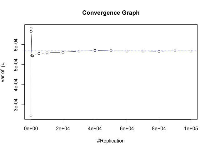
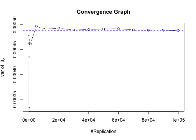
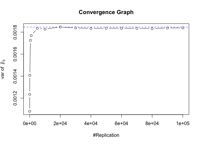
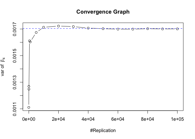
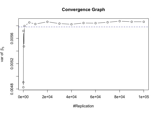
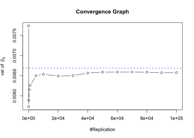
Plot of variance of betahat

# beta - betahat ~ N(0, sigma^2 (X^T X)^-1)
var.beta <- sig2e*solve(t(X)%*%X)
foo2 = expression("var of "~hat(beta)[1], 
                  "var of "~hat(beta)[2],
                  "var of "~hat(beta)[3],
                  "var of "~hat(beta)[4],
                  "var of "~hat(beta)[5],
                  "var of "~hat(beta)[6])
for (i in 1:length(beta)){
  # mypath <- file.path(getwd(),"Figure",paste("i_var_betahat_",i, ".jpeg", sep = ""))
  # jpeg(mypath, height = 8, width = 8, units = 'in', res = 300)
  plot(vecN, mat.vebh[,i], 
       type="b", xlab = "#Replication", 
       ylab = foo2[[i]], main="Convergence Graph")
  abline(h=var.beta[i,i], col = "blue", lty = 2)
  # dev.off()
}

The difference between true value and the last similated value

1	abs(diag(var.beta)-mat.vebh[length(vecN),])

##                      rmrf          smb          hml          rmw 
## 1.275990e-06 3.146077e-07 7.275822e-06 2.791952e-06 8.092901e-05 
##          cma 
## 1.124775e-04

Plot of error variance

# Error Variance
# Unbised estimater of sigma^2
# mypath <- file.path(getwd(),"Figure","i_var_err.jpeg")
# jpeg(mypath, height = 8, width = 8, units = 'in', res = 300)
plot(vecN, vec.err.varh, type="b", xlab = "#Replication", ylab = "Error Var.")
abline(h=sig2e, col = "blue", lty = 2)

1	# dev.off()

The difference between true value and the last similated value:

1	abs(sig2e-vec.err.varh[length(vecN)])

## [1] 4.572658e-05

Finding (ii)

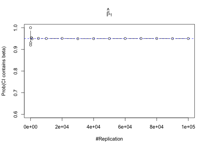
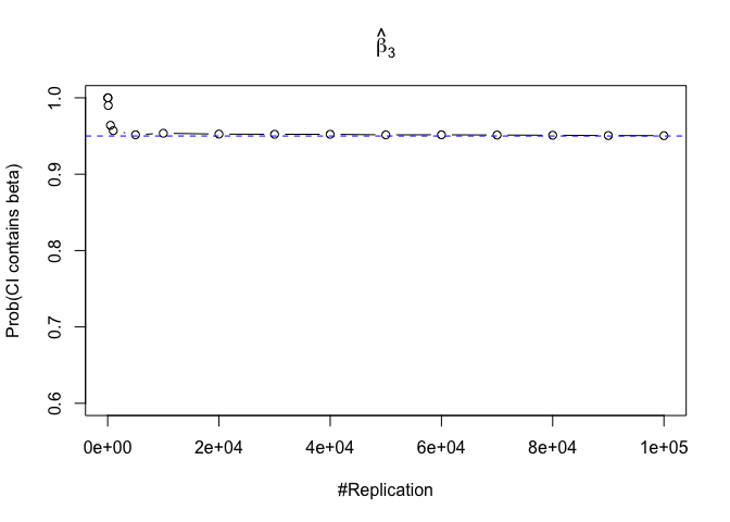
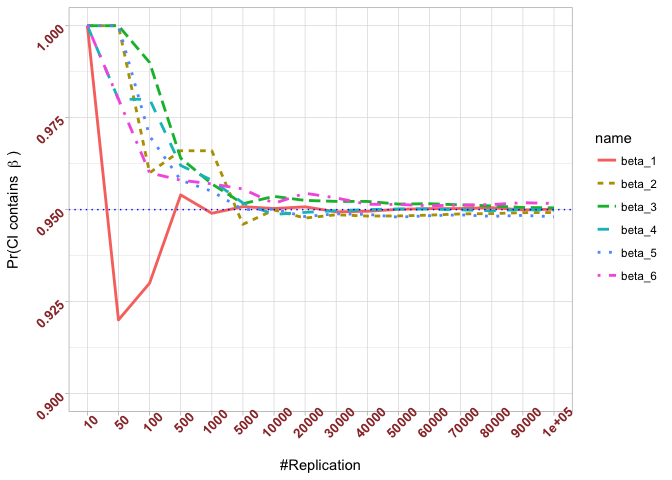
The “correct” meaning of a 100(1‐α)% confidence interval of an unknown coefficient

for (i in 1:length(beta)){
  # mypath <- file.path(getwd(),"Figure",paste("ii_prob_beta_",i, ".jpeg", sep = ""))
  # jpeg(mypath, height = 8, width = 8, units = 'in', res = 300)
  plot(vecN, prob.flag.beta[,i], type="b", xlab = "#Replication", ylab = "Prob(CI contains beta)", main=foo[[i]], ylim = c(0.6,1))
  abline(h=0.95, col = "blue", lty = 2)
  # dev.off()
}

Plot in one graph:

# in one graph
mydimnames <- list(vecN, name=c("beta_1", "beta_2", "beta_3",
                                "beta_4", "beta_5", "beta_6"))
dimnames(prob.flag.beta)=mydimnames
tempdata <- as.data.frame(as.table(prob.flag.beta))
library(ggplot2)
ggplot(data = tempdata, aes(x = Var1, y=Freq, group = name)) + 
  geom_line(aes(linetype=name, color = name), size=1) + 
  xlab("#Replication") + 
  ylab(expression("Pr(CI contains "~beta~")")) + 
  ylim(0.9,1) + 
  geom_hline(yintercept = .95, color = "blue", linetype="dotted") +
  theme_light() +
  theme(axis.text.x = element_text(face="bold", color="#993333", 
                                   size=10, angle=45),
        axis.text.y = element_text(face="bold", color="#993333", 
                                   size=10, angle=45))

The difference between true value and the last similated value

1	abs(0.95-prob.flag.beta[length(vecN),])

##  beta_1  beta_2  beta_3  beta_4  beta_5  beta_6 
## 0.00012 0.00079 0.00048 0.00018 0.00194 0.00167

Finding (iii)

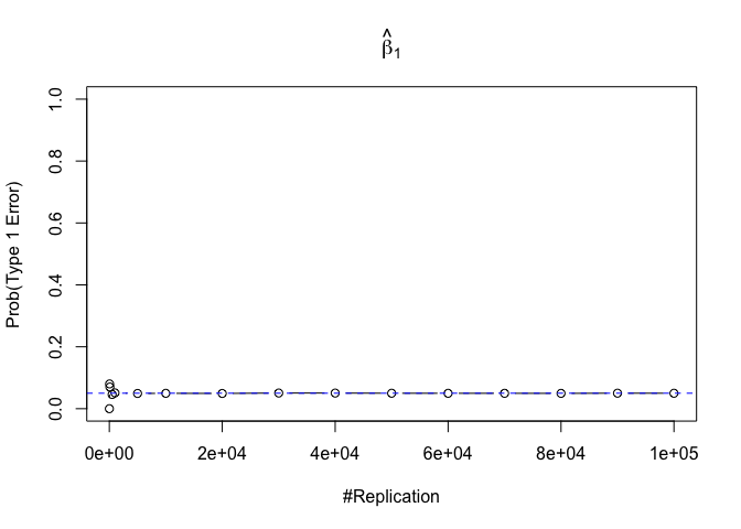
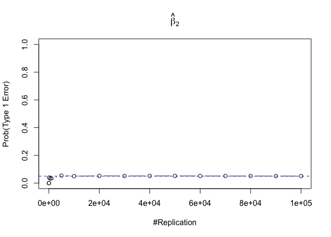
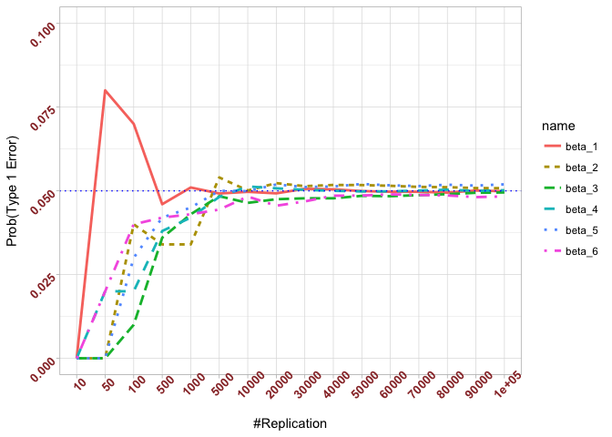
The significance level of the t test for testing a linear hypothesis concerning one or more coefficients is the probability of committing a Type I error

for (i in 1:length(beta)){
  # mypath <- file.path(getwd(),"Figure",paste("iii_prob_type1err_",i, ".jpeg", sep = ""))
  # jpeg(mypath, height = 8, width = 8, units = 'in', res = 300)
  plot(vecN, prob.flag.type1[,i],
       type="b", xlab = "#Replication", 
       ylab = "Prob(Type 1 Error)", 
       main=foo[[i]], ylim = c(0,1))
  abline(h=0.05, col = "blue", lty = 2)
  # dev.off()
}

Plot in one graph:

# in one graph
mydimnames <- list(vecN, name=c("beta_1", "beta_2", "beta_3", 
                                "beta_4", "beta_5", "beta_6"))
dimnames(prob.flag.type1)=mydimnames
tempdata <- as.data.frame(as.table(prob.flag.type1))
library(ggplot2)
ggplot(data = tempdata, aes(x = Var1, y=Freq, group = name)) + 
  geom_line(aes(linetype = name, color = name), size = 1) + 
  xlab("#Replication") + 
  ylab("Prob(Type 1 Error)") + 
  ylim(0,0.1) + 
  geom_hline(yintercept = .05, color = "blue", linetype = "dotted")+
  theme_light() +
  theme(axis.text.x = element_text(face="bold", color="#993333", 
                                   size=10, angle=45),
        axis.text.y = element_text(face="bold", color="#993333", 
                                   size=10, angle=45))

The difference between true value and the last similated value

1	abs(0.05-prob.flag.type1[length(vecN),])

##  beta_1  beta_2  beta_3  beta_4  beta_5  beta_6 
## 0.00012 0.00079 0.00048 0.00018 0.00194 0.00167

Finding (iv)

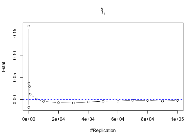
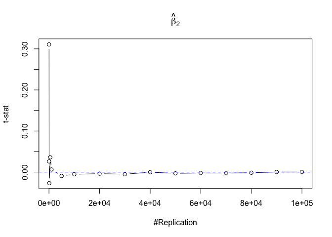
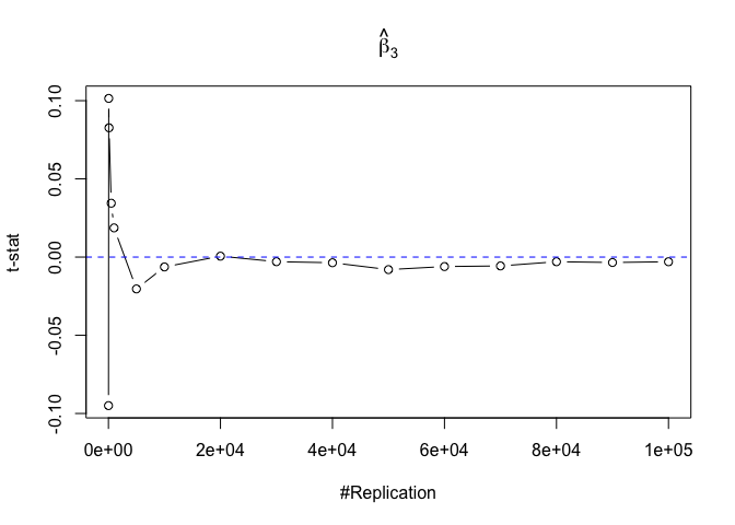
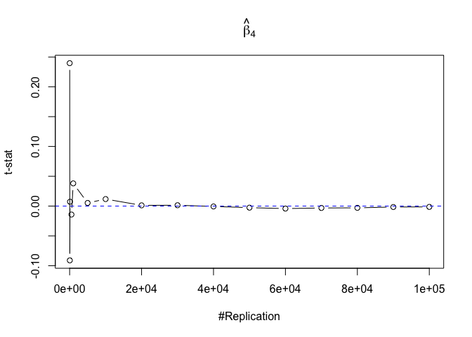
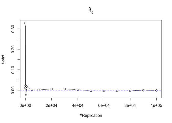
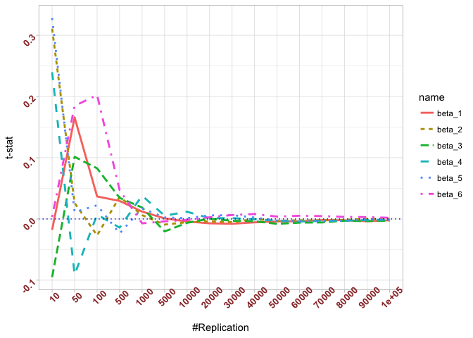
The t test is unbiased

for (i in 1:length(beta)){
  # mypath <- file.path(getwd(),"Figure",paste("iv_tstat_",i, ".jpeg", sep = ""))
  # jpeg(mypath, height = 8, width = 8, units = 'in', res = 300)
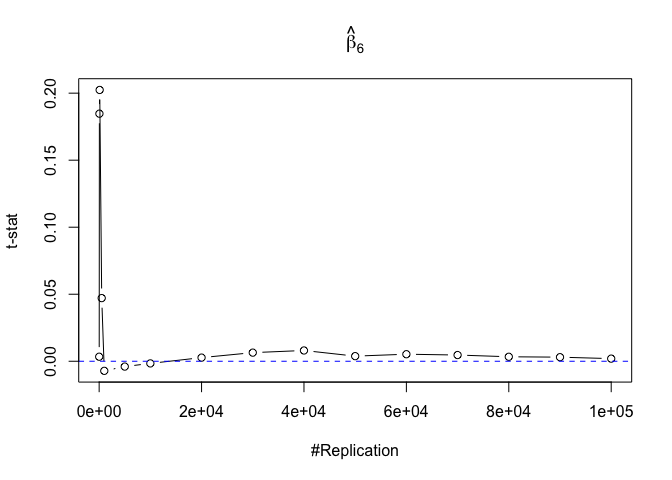
  plot(vecN, mat.t.stathat[,i], type="b", xlab = "#Replication", ylab = "t-stat", main=foo[[i]])
  abline(h=0, col = "blue", lty = 2)
  # dev.off()
}

Plot in one graph:

# in one graph
mydimnames <- list(vecN, name=c("beta_1", "beta_2", "beta_3", 
                                "beta_4", "beta_5", "beta_6"))
dimnames(mat.t.stathat)=mydimnames
tempdata <- as.data.frame(as.table(mat.t.stathat))
library(ggplot2)
ggplot(data = tempdata, aes(x = Var1, y=Freq, group = name)) + 
  geom_line(aes(linetype = name, color = name), size = 1) + 
  xlab("#Replication") + 
  ylab("t-stat") + 
  geom_hline(yintercept = 0, color = "blue", linetype = "dotted") +
  theme_light() +
  theme(axis.text.x = element_text(face="bold", color="#993333", 
                                   size=10, angle=45),
        axis.text.y = element_text(face="bold", color="#993333", 
                                   size=10, angle=45))

The difference between true value and the last similated value

1	abs(0-mat.t.stathat[length(vecN),])

##       beta_1       beta_2       beta_3       beta_4       beta_5 
## 0.0021438691 0.0002507301 0.0029878315 0.0013417811 0.0013706685 
##       beta_6 
## 0.0019628747

Finding (v)

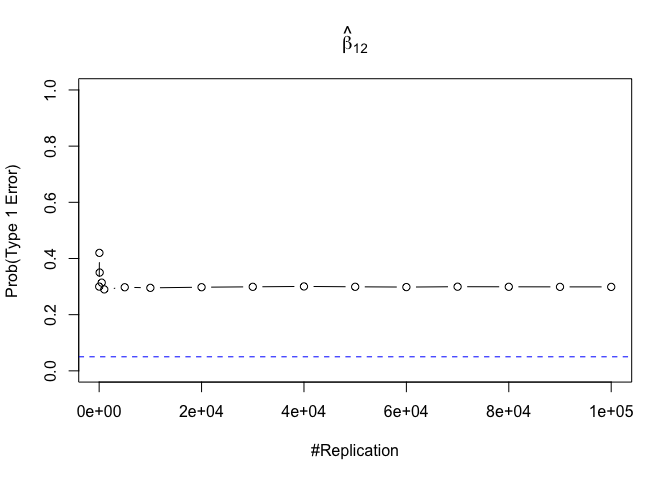
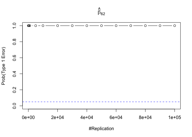
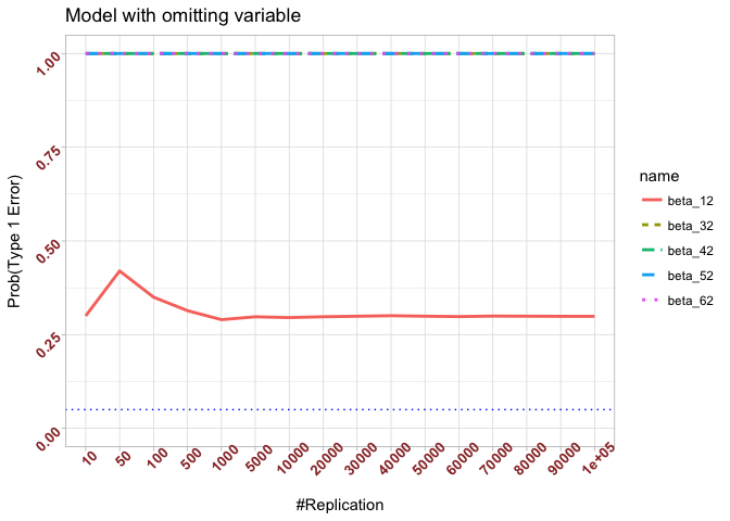
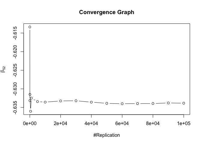
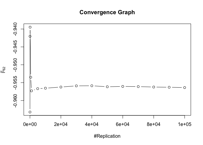
The result in Part iii) no longer holds if some relevant explanatory variables have been omitted from the model

We omitt the variable rmrf (K_m − R_f).

foo3 = expression(hat(beta)[12], hat(beta)[32],hat(beta)[42],hat(beta)[52],hat(beta)[62])
for (i in 1:(length(beta)-1)){
  # mypath <- file.path(getwd(),"Figure",paste("v_prob_type1err_",i, ".jpeg", sep = ""))
  # jpeg(mypath, height = 8, width = 8, units = 'in', res = 300)
  plot(vecN, prob.flag.type1.2[,i], type="b", xlab = "#Replication", ylab = "Prob(Type 1 Error)", main=foo3[[i]], ylim = c(0,1))
  abline(h=0.05, col = "blue", lty = 2)
  # dev.off()
}

# in one graph
mydimnames <- list(vecN, name=c("beta_12", "beta_32", 
                                "beta_42", "beta_52", "beta_62"))
dimnames(prob.flag.type1.2)=mydimnames
tempdata <- as.data.frame(as.table(prob.flag.type1.2))
library(ggplot2)
ggplot(data = tempdata, aes(x = Var1, y=Freq, group = name)) + 
  geom_line(aes(linetype = name, color = name), size = 1) + 
  xlab("#Replication") + 
  ylab("Prob(Type 1 Error)")+ 
  ylim(0,1) + 
  geom_hline(yintercept = 0.05, color = "blue", linetype = "dotted") +
  ggtitle("Model with omitting variable") +
  theme_light() +
  theme(axis.text.x = element_text(face="bold", color="#993333", 
                                   size=10, angle=45),
        axis.text.y = element_text(face="bold", color="#993333", 
                                   size=10, angle=45))

The difference between true value and the last similated value

1	abs(0.05-prob.flag.type1.2[length(vecN),])

## beta_12 beta_32 beta_42 beta_52 beta_62 
## 0.24885 0.94999 0.95000 0.95000 0.95000

Finding (vi)

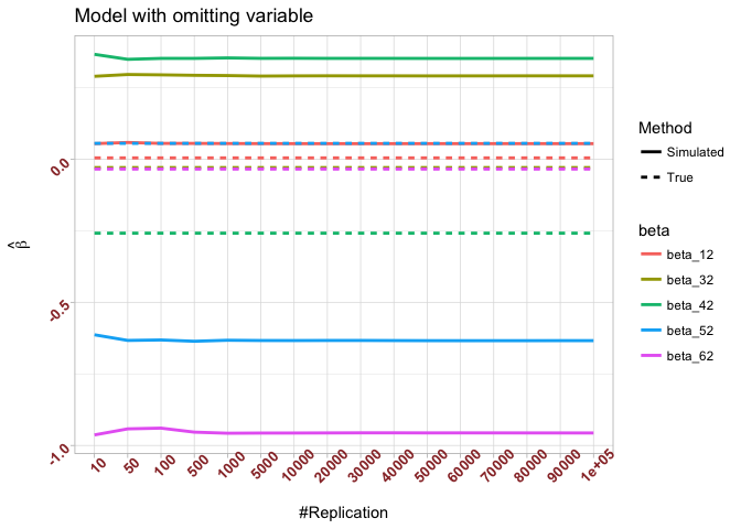
The estimator of say, the coefficient of X2, is no longer unbiased if the decision of whether to include X1 in the model is dependent on the outcome of a t test. Based on your findings, discuss the wider implications of “model selection” for statistical modeling and the lessons to be learnt for practitioners.

Plot of betahat of omitting model

temp <- 1:length(beta)
nbv <- temp[-2]
for (i in 1:(length(beta)-1)){
  # mypath <- file.path(getwd(),"Figure",paste("vi_batahat_",i, ".jpeg", sep = ""))
  # jpeg(mypath, height = 8, width = 8, units = 'in', res = 300)
  plot(vecN, mat.betahat2[,i], type="b", xlab = "#Replication", ylab = foo3[[i]], main="Convergence Graph")
  abline(h=beta[nbv[i]], col = "blue", lty = 2)
  # dev.off()
}

# One graph
#
mydimnames1 <- list(vecN, 
                    name=c("beta_12", "beta_32", 
                           "beta_42", "beta_52", "beta_62"))
dimnames(mat.betahat2)=mydimnames1
#
mydimnames2 <- list(vecN, 
                    name=c("beta_12", "beta_32", 
                           "beta_42", "beta_52", "beta_62"))
trueb <- t(replicate(length(vecN),beta[nbv]))
dimnames(trueb)=mydimnames2
#
method = gl(2,(length(beta)-1)*length(vecN),
            (length(beta)-1)*length(vecN)*2, 
            labels = c("Simulated", "True")) 
tempdata <- as.data.frame(as.table(cbind(mat.betahat2,trueb)))
colnames(tempdata) <- c("N","beta","Value")
tempdata$Method <- method

library(ggplot2)
ggplot(data = tempdata, aes(x = N, y = Value, 
                            linetype = Method, colour = beta, 
                            group = interaction(beta, Method))) +
  geom_line(size = 1) + 
  xlab("#Replication") + 
  ylab(expression(hat(beta))) + 
  ggtitle("Model with omitting variable") +
  theme_light() +
  theme(axis.text.x = element_text(face="bold", color="#993333", 
                                   size=10, angle=45),
        axis.text.y = element_text(face="bold", color="#993333", 
                                   size=10, angle=45))

The difference between true value and the last similated value

1	abs(beta[nbv]-mat.betahat2[length(vecN),])

## (Intercept)         smb         hml         rmw         cma 
##  0.04978255  0.32050856  0.61052734  0.68909783  0.92192545

Plot of Error Variance of omitting model

Unbised estimater of sigma^2

# mypath <- file.path(getwd(),"Figure","vi_var_err.jpeg")
# jpeg(mypath, height = 8, width = 8, units = 'in', res = 300)
# bty for Box Style
plot(vecN, vec.err.varh2, type="b", xlab = "#Replication", ylab = "Error Var.", main = "Model of omitting")
abline(h=sig2e, col = "blue", lty = 2)

1	# dev.off()

The difference between true value and the last similated value

1	abs(sig2e-vec.err.varh2[length(vecN)])

## [1] 1.113663

Reference

Monte Carlo Method

Monte Carlo Methods Lecture Notes by Adam M. Johansen and Ludger Evers, November 15, 2007
Machine Learning: The elegant way to extract information from data: Lecture notes on Regression: Markov Chain Monte Carlo (MCMC)
- All Slides
Monte Carlo Simulation Basics, I: Historical Notes
Monte Carlo Simulation Basics, II: Estimator Properties
Monte Carlo Simulation Basics, III: Regression Model Estimators

Welcome!

Monte Carlo Experiment for Fama French 5 Factor Model

Model

Data Source

Fama/French 3 Factors [Daily]

Portfolios Formed on Book-to-Market [Daily]

Load Data

Extract Fama-French Factors and Fund Returns

Run Fama-French Regression

Monte Carlo Simulation

One example of Monte Carlo Simulation

Running Monte Carlo Simulation

Plot

Plot of density of estimator

Finding (i)

Plot of betahat

Plot of variance of betahat

Plot of error variance

Finding (ii)

Finding (iii)

Finding (iv)

Finding (v)

Finding (vi)

Plot of betahat of omitting model

Plot of Error Variance of omitting model

Reference

Monte Carlo Method

Fama French Model

Intro

Tutorial